Welcome to Geotech!
Exploring High‑Precision Magnetic Field Meters: Applications of Proton Magnetometers
From the early 20th century to the present, magnetometers have undergone remarkable evolution—from simple mechanical devices to highly sophisticated instruments based on advanced physics and electronics. Today, the three most widely used high‑precision magnetometers are the Proton Magnetometer, the Optically Pumped Magnetometer, and the Fluxgate Magnetometer.
Magnetometer Classifications
Magnetometers can be classified by their historical development and the physical principles on which they operate:
- First Generation
- Relied on permanent magnets interacting with Earth’s field or induction coils plus mechanical components.
- Examples: mechanical magnetometers, airborne induction magnetometers.
- Second Generation
- Use nuclear magnetic resonance and complex electronics.
- Examples: Proton Magnetometers, Optically Pumped Magnetometers, Fluxgate Magnetometers.
- These are today’s most widespread high‑precision instruments.
- Third Generation
- Based on low‑temperature quantum effects.
- Example: SQUID (Superconducting Quantum Interference Device) magnetometers.
- Fourth Generation
- Under active research; exploit atomic quantum states for ultra‑high sensitivity.
- Example: Atomic magnetometers.
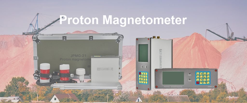
In practical geophysical work, Proton Magnetometers and Optically Pumped Magnetometers dominate. Although Optically Pumped Magnetometers offer very high precision, they tend to be heavy, expensive, and power‑hungry—making them ideal for airborne surveys. By contrast, Proton Magnetometers are lightweight, stable, and sufficiently sensitive for high‑precision ground surveys.
1. Principle of Proton Magnetometers
1.1 Historical Background
In 1954, Packard and Varian proposed measuring Earth’s magnetic field by observing the precession frequency of hydrogen nuclei in water. The following year, U.S. researchers built the first working Proton Magnetometer. Inside its probe, a hydrogen‑rich sample (e.g., water) is polarized by a strong static magnetic field (~100 gauss, or 0.01 T). Once the polarization field is removed, the hydrogen nuclei precess around Earth’s field direction. Their Larmor precession frequency fff is linearly related to magnetic field strength BBB by f=γBf = \gamma Bf=γB
where γ\gammaγ (the gyromagnetic ratio of the proton) is approximately 42.576 MHz/T. By measuring this frequency, the ambient magnetic field strength can be directly determined. Computing the signal amplitude then involves Boltzmann statistics and other advanced physics.
1.2 Detecting the Larmor Frequency
We detect the proton precession via Faraday’s law of induction: changing magnetic flux through a coil induces an electromotive force. When the precessing protons act like tiny magnets, their changing flux in a sensitive coil produces a voltage oscillating at the Larmor frequency. By measuring that oscillation, the instrument infers the magnetic field intensity.
2. Operating Procedure
- Polarization
- Apply a strong auxiliary field to align (“polarize”) the proton spins.
- Measurement
- Quickly switch off the auxiliary field.
- Use a dedicated induction coil to capture the proton precession signal.
- Frequency Analysis
- Convert the induced voltage oscillation into a frequency measurement.
- Calculate the magnetic field strength from the known proton gyromagnetic ratio.
3. Applications of Proton Magnetometers
- Mineral Exploration:
High‑precision detection of ferromagnetic ore bodies (e.g., magnetite, hematite). - Hydrocarbon Basin Screening:
Mapping subtle structural anomalies in oil‑ and gas‑bearing formations. - Engineering and Environmental Surveys:
Locating buried objects, assessing fill materials, and guiding safe construction. - Pipeline and Utility Detection:
Non‑intrusive mapping of underground steel pipes and reinforcing components. - Archaeology:
High‑resolution mapping of buried foundations and cultural relics through magnetic anomalies.
4. Major Manufacturers and Comparative Overview
| Manufacturer / Model | Absolute Accuracy | Sampling Rate | Key Features |
|---|---|---|---|
| Geometric / Geometrics (USA) | ±0.2 nT | 0.5–60 s per reading | Industry‑standard field units |
| GEM Systems (Canada) | ±0.1–0.2 nT | 0.5–60 s per reading | “Walking Mag” mode, cost‑effective |
| PGM (Czech Republic) | ±0.1 nT | 2–10 s per reading | Compact, high stability |
| Overhauser Magnetometers | ±0.01 nT | ≤ 0.2 s per reading | Ultra‑high sensitivity, low power consumption |
| Fluxgate Magnetometers | ±1–10 nT | Real‑time | Lightweight, low cost—ideal for UAV/vehicle use |
Domestic R&D in Proton Magnetometers began later and often lags in features and reliability compared to these established international brands.
5. Why Choose a Proton Magnetometer?
- Simplicity & Reliability: Fewer moving parts and robust electronics make maintenance easier.
- Cost‑Effectiveness: Generally lower purchase and operating costs than optically pumped or SQUID systems.
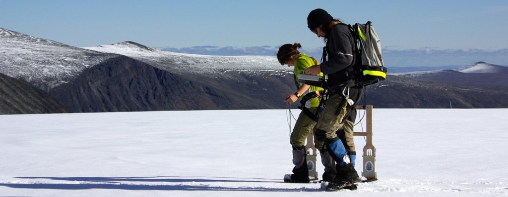
- Portability: Field‑ready units that one person can carry over rugged terrain.
- Adequate Sensitivity: Precision down to tenths of a nanotesla meets most geophysical and archaeological requirements.
6. Future Trends
- Fourth‑Generation Atomic Magnetometers: Aim for picotesla‑level sensitivity at room temperature.
- Multi‑Sensor Fusion: Integrating magnetic, electrical, and seismic data for richer subsurface imaging.
- UAV‑Borne Surveys: Lightweight magnetometer packages enabling rapid, wide‑area reconnaissance.
- AI‑Assisted Inversion: Machine learning algorithms to convert field data into detailed 3D models.
As domestic manufacturers continue to advance, the gap with international leaders is narrowing. We can expect high‑precision, low‑cost Proton Magnetometers to become even more widely accessible, driving innovation across mineral exploration, archaeology, and engineering geophysics.
Reference
- WIKI:https://en.wikipedia.org/wiki/Electrical_resistivity_tomography
- Society of Exploration Geophysicists (SEG) https://seg.org/
- Society of Environmental and Engineering Geophysicists (EEGS) https://www.eegs.org/
- Geology and Equipment Branch of China Mining Association http://www.chinamining.org.cn/
- International Union of Geological Sciences (IUGS) http://www.iugs.org/
- European Geological Survey Union (Eurogeosurveys) https://www.eurogeosurveys.org/