What Is Continuous Resistivity Profiling? Principle, Equipment and Applications

Overview：Continuous resistivity profiling (CRP) is a waterborne geophysical technique that maps sub-bottom electrical resistivity via towed electrode streamers. Continuous resistivity profiling delivers high-efficiency subsurface imaging for estuarine, riverine and lacustrine environments, supporting submarine groundwater discharge detection, sediment characterization and bedrock mapping.

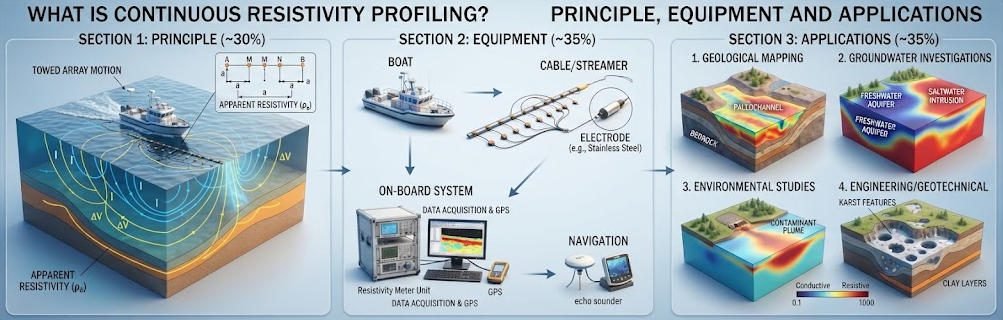
Ⅰ. Definition and Fundamental Principle

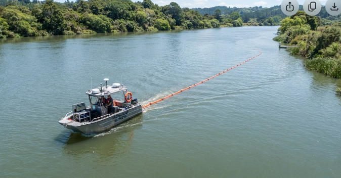
1. Core Definition

Continuous Resistivity Profiling (CRP) is a waterborne direct-current (DC) resistivity method that images sub-surface electrical properties beneath rivers, estuaries, lakes and coastal waters. It uses a towed multi-electrode cable to acquire apparent resistivity data continuously along a survey trackline.

Unlike land-based resistivity surveys with stationary electrodes, CRP operates from a moving vessel. It generates a continuous two-dimensional cross-section of subsurface resistivity beneath the water-sediment interface. Typical investigation depths range from a few meters to approximately 25 percent of the streamer length, depending on array configuration and water conductivity.

CRP is sometimes referred to as waterborne electrical resistivity tomography (ERT) or towed resistivity surveying. It shares the same physical foundation as land ERT but adopts a mobile acquisition geometry optimized for aquatic environments.

2. Basic Physical Principle

CRP operates on the principle of electrical resistivity. When direct current is injected into water and sub-bottom sediments through two source electrodes, it creates an electric field in the subsurface. The distribution of this field depends on the resistivity of underlying geological materials and pore fluids.

Potential electrodes located along the streamer measure voltage differences caused by the injected current. Apparent resistivity is calculated from the measured voltage, injected current and geometric factor of the electrode array. Resistivity values reflect lithology, porosity, pore-fluid salinity and saturation.

Fresh groundwater typically exhibits high resistivity, while saline water and clay-rich sediments show low resistivity. This contrast enables CRP to map fresh-saline water interfaces, sedimentary layers and buried geological features.

Ⅱ. System Equipment and Field Acquisition Workflow

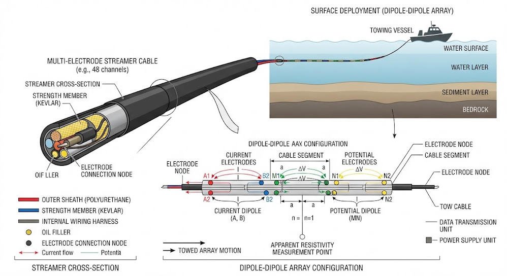
1. System Hardware Configuration

A standard CRP system consists of four core components: resistivity meter, electrode streamer, navigation and bathymetry unit, and survey vessel.

Component	Description	Typical Specifications
Resistivity transmitter/receiver	Controls current injection and voltage sampling	8–16 channels, 100–500 W output power, 2–5 s sampling interval
Electrode streamer	Floating cable with evenly spaced electrodes	15–100 m length, 11 electrodes, 1.5–10 m electrode spacing
Navigation system	GPS positioning and track recording	Sub-meter accuracy, synchronized with resistivity data
Bathymetric transducer	Measures water depth and temperature	200 kHz single-beam sounder

The streamer carries two current electrodes near the vessel and multiple potential electrodes further aft. Graphite is commonly used for current electrodes to minimize polarization effects, while stainless steel is standard for potential electrodes. Foam floats along the cable maintain electrode depth near the water surface.

2. Standard Field Acquisition Procedure

CRP surveys follow a structured workflow to ensure data quality and positional accuracy.

First, the survey team calibrates the resistivity system and verifies electrode continuity before deployment. The streamer is deployed from the stern of the survey vessel, with layback offset measured and recorded for later position correction.

The vessel travels at a constant slow speed, typically 2–5 km/h, along pre-planned tracklines. The system injects DC current pulses and records voltage measurements at fixed time intervals. Each measurement cycle produces a full set of dipole-dipole or Wenner array readings.

GPS coordinates, water depth and water temperature are logged synchronously with resistivity data. Survey speed is adjusted to ensure sufficient spatial sampling, usually one measurement every 3–5 meters along track.

3. Data Processing and Inversion

Raw CRP data requires preprocessing before geological interpretation. The workflow includes bad data removal, drift correction, geometric factor calculation and apparent resistivity computation.

Water column resistivity and bathymetry are applied as constraints during inversion to improve model accuracy. Inversion software converts apparent resistivity pseudosections into true resistivity cross-sections using smoothness-constrained least-squares algorithms.

Final deliverables typically include 2D resistivity profiles, GIS-compatible trackline data and interpreted geological sections. Advanced projects integrate CRP with continuous seismic profiling for joint interpretation.

Ⅲ. CRP vs. Conventional Land ERT: Comparative Analysis

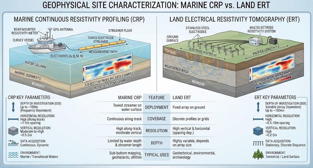
CRP and land ERT share the same electrical principle but differ significantly in deployment, resolution and project efficiency.

Technical Parameter	Continuous Resistivity Profiling (CRP)	Conventional Land ERT
Deployment mode	Towed from moving vessel, continuous acquisition	Stationary electrode array, discrete measurements
Typical array	Dipole-dipole (fixed along streamer)	Wenner, Schlumberger, dipole-dipole, pole-pole
Depth of investigation	~20–25% of streamer length	Up to hundreds of meters with large arrays
Lateral sampling	Continuous along track, ~3–5 m spacing	Discrete at electrode locations
Survey speed	2–5 km of profile per hour	0.5–2 km of profile per day
Vertical resolution	Decreases rapidly with depth	Better vertical control with multi-array designs
Primary environment	Rivers, estuaries, lakes, shallow coastal waters	Land-based engineering, environmental, mining sites

CRP achieves much higher line-kilometer productivity than land ERT in aquatic settings. It eliminates the need for manual electrode placement and allows coverage of large survey areas in days rather than weeks.

However, land ERT offers greater flexibility in array design and deeper penetration. It also supports reciprocal measurements for error quantification, which is generally impractical with towed CRP systems.

Ⅳ. Major Application Domains

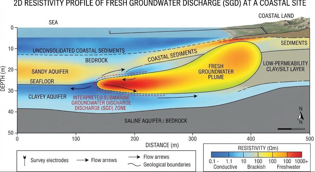
1. Submarine Groundwater Discharge (SGD) Mapping

SGD mapping is the most widespread application of continuous resistivity profiling. Fresh groundwater discharging into coastal waters has higher resistivity than ambient seawater, creating a detectable electrical anomaly.

CRP can image low-salinity groundwater plumes extending tens to hundreds of meters offshore. It reveals the geometry of the fresh-saline interface and identifies preferential discharge pathways along buried paleochannels.

This application supports coastal water quality management, nutrient loading assessment and eutrophication risk evaluation. It provides spatially continuous data that complements discrete point measurements from piezometers and seepage meters.

2. Sediment Classification and Bedrock Detection

Resistivity contrasts between unconsolidated sediments and bedrock allow CRP to map sediment thickness and bedrock topography. Coarse-grained sediments generally have higher resistivity than fine-grained muds and clays.

CRP surveys are routinely used for reservoir sedimentation assessment, river channel morphology studies and dam impoundment surveys. They provide continuous bedrock depth profiles along entire river reaches with minimal field effort.

In dredging and navigation projects, CRP delivers rapid pre-construction characterization of sub-bottom conditions. It helps identify buried obstacles and estimates sediment volumes for removal.

3. Hydrogeological Investigations

In riverine and lacustrine environments, CRP supports aquifer characterization and groundwater-surface water interaction studies. It maps hydraulic conductivity variations and identifies gaining and losing reaches.

Time-lapse CRP surveys can monitor seasonal changes in groundwater levels and salinity distribution. They provide insights into hyporheic exchange processes and bank storage dynamics.

Combined with borehole data, CRP data improves the calibration of groundwater flow models. It adds spatial continuity to point-based hydrogeological measurements.

4. Environmental Site Assessment

CRP detects and maps conductive contaminant plumes in underwater sediments. Landfill leachate, industrial effluents and saline intrusion create measurable resistivity anomalies.

The method can also locate buried waste objects and pipeline routes beneath water bodies. It provides a non-invasive screening tool before intrusive sediment sampling.

For long-term monitoring programs, repeat CRP surveys track plume migration and remediation progress. They offer cost-effective coverage of large contaminated water bodies.

Ⅴ. Limitations and Quality Control Considerations

1. Inherent Method Limitations

CRP shares the fundamental limitations of surface resistivity methods. Vertical resolution decreases with depth, and deep features appear smoother and less defined than shallow features.

The effective depth of investigation is limited to approximately 20–25 percent of the streamer length. Longer streamers reach deeper but sacrifice horizontal resolution and maneuverability in narrow waterways.

Non-uniqueness is another inherent constraint. Different geological combinations can produce identical resistivity responses. Interpretation must always be calibrated with local geological knowledge and ground-truth data.

2. Field Noise Sources and Mitigation

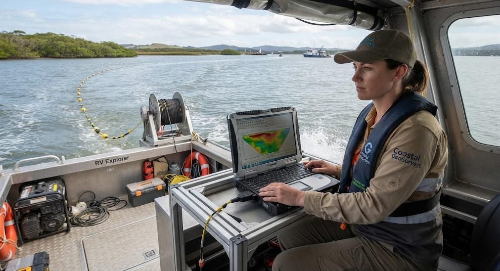
Several field factors can degrade CRP data quality. Boat speed variations cause uneven spatial sampling and signal stacking inconsistencies. Optimal survey speed depends on system sampling rate and required data density.

Water column conductivity variations introduce errors if not properly measured and corrected. Temperature and salinity profiles should be collected at regular intervals during the survey.

Vegetation entanglement, bottom contact and lateral streamer drift can produce measurement artifacts. Survey design should account for tidal stages, current patterns and weather windows to minimize these effects.

Rigorous quality control includes real-time data monitoring, post-survey noise filtering and comparison with independent datasets such as seismic profiles and borehole logs.

Ⅵ. Project Design Best Practices

Successful CRP projects require careful planning matched to project objectives and site conditions.

First, define the target depth and required resolution. Select streamer length and electrode spacing accordingly. Shallow high-resolution surveys use 15 m streamers with 1.5 m spacing, while deep regional surveys use 50–100 m streamers.

Second, design trackline layout based on geological strike. Lines should be oriented perpendicular to expected geological features and flow paths. Grid patterns are used for 3D interpretation in complex areas.

Third, plan for ground-truthing. Reserve budget for targeted sediment sampling or borehole verification at key anomaly locations. No resistivity survey should be interpreted without geological calibration.

Finally, consider complementary methods. Combining CRP with continuous seismic profiling produces more robust interpretations than either method alone. Electromagnetic methods can provide additional reconnaissance data for project scoping.

---

Related Articles

Title	Core Content	URL
What is Vertical Electrical Sounding (VES)?	Explains DC resistivity sounding principle, Schlumberger array, and applications in groundwater and bedrock mapping	https://geotechcn.net/service/what-is-ves-ert-systems/
2D vs 3D ERT: Complete Field Guide	Compares 2D and 3D electrical resistivity tomography workflows, equipment, resolution and cost structures	https://geotechcn.net/service/2d-vs-3d-electrical-resistivity-imaging-methods/
Comparative Study of Geophysical Exploration Methods: HDR, ERT & DC	Analyzes DC resistivity sounding, ERT and high-density resistivity methods with field case examples	https://geotechcn.net/service/hdr-vs-ert-vs-dc-sounding-geophysical-method-guide/
Principle of High-Density Electrical Resistivity Survey and Case Analysis	Details high-density resistivity system architecture, inversion algorithms and engineering geology applications	https://geotechcn.net/service/electrical-method/
What Are Electrical and Electromagnetic Equipment in Geophysical Surveys?	Covers electrode array configurations, resistivity imaging systems and electromagnetic survey equipment	https://geotechcn.net/service/electrical-vs-electromagnetic-survey/

Reference Sources

Title	Core Content	URL
Continuous Resistivity Profiling	EPA technical guide covering CRP principles, applications, limitations and data interpretation practices	https://19january2025snapshot.epa.gov/environmental-geophysics/continuous-resistivity-profiling/index.html
Continuous Resistivity Profiling and Seismic-Reflection Data, Indian River Bay	USGS field dataset with system specifications, survey methodology and processed resistivity results	https://pubs.usgs.gov/of/2011/1039/html/ofr2011-1039-glossary.html
Continuous resistivity profiling to delineate submarine groundwater discharge	Peer-reviewed research paper on CRP methodology, inversion and SGD case studies	https://pubs.geoscienceworld.org/seg/tle/article/25/6/724/135270/Continuous-resistivity-profiling-to-delineate
Estimation of Impounded Sediment Volume with Continuous Resistivity Profiling	USGS case study applying CRP to sediment volume calculation in dam impoundments	https://pubs.usgs.gov/publication/sir20265126/full
Waterborne Resistivity Survey Methods, Northport Harbor	USGS methods documentation for CRP equipment configuration, data acquisition and processing workflows	https://pubs.usgs.gov/of/2011/1041/html/methods.html

---

FAQ