Welcome to Geotech!



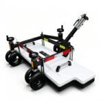
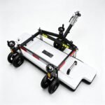
Vehicle‑Mounted 3D Array Ground Penetrating Radar丨GEO‑GPR‑3D‑V




PRODUCT PARAMETERS
Description
 Abstract
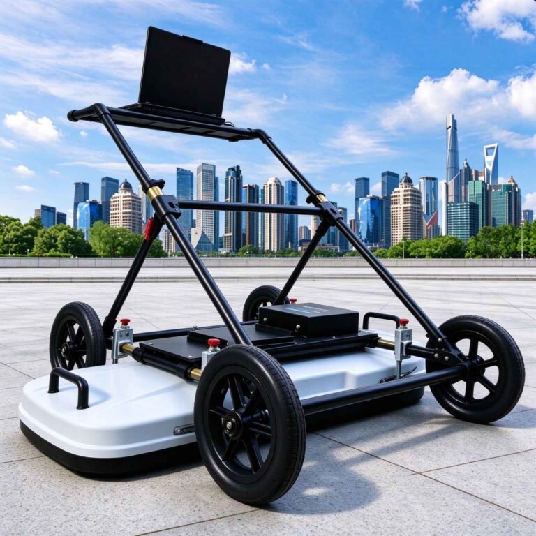
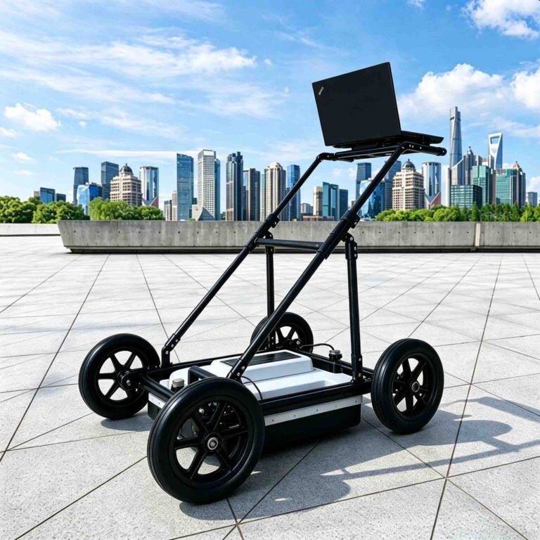
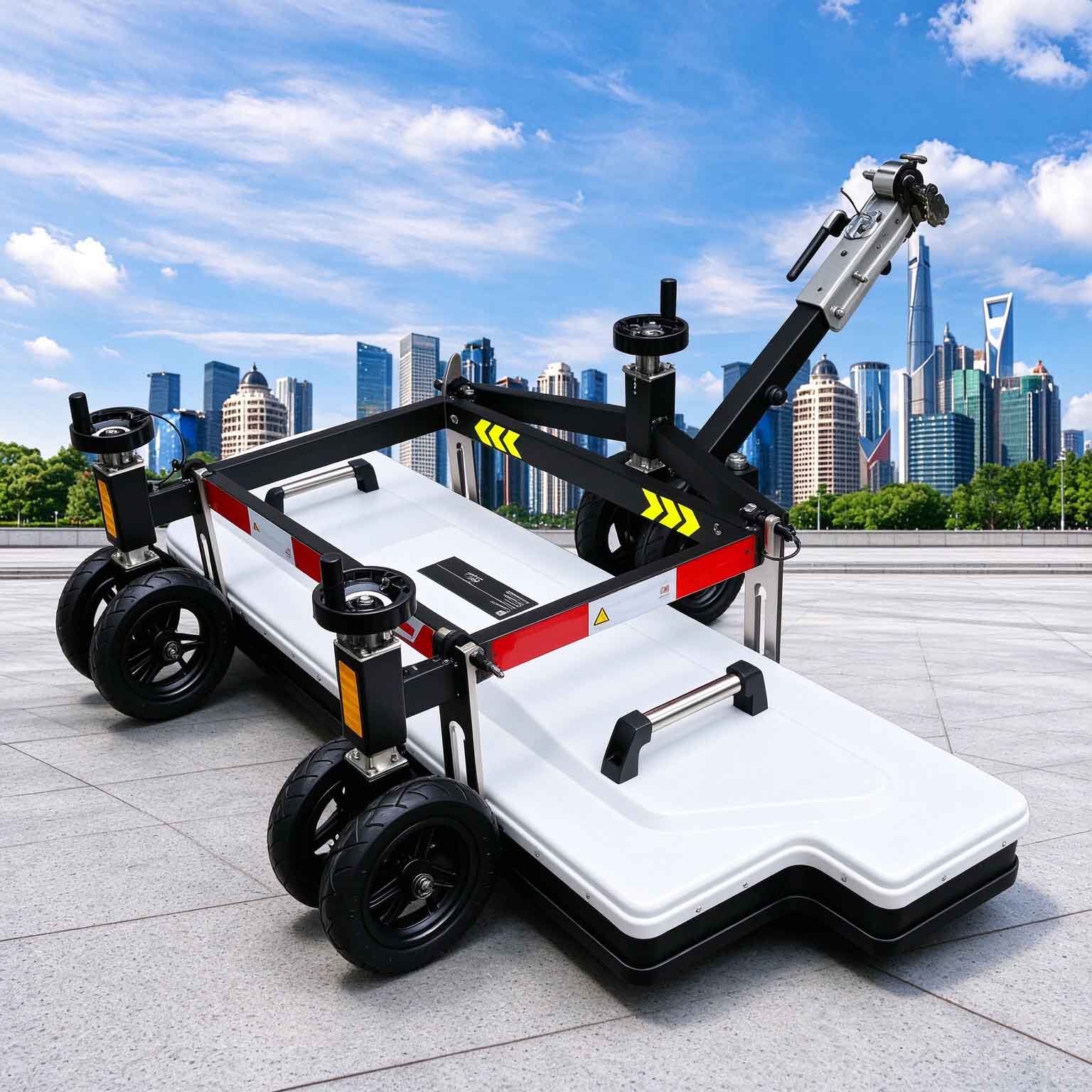
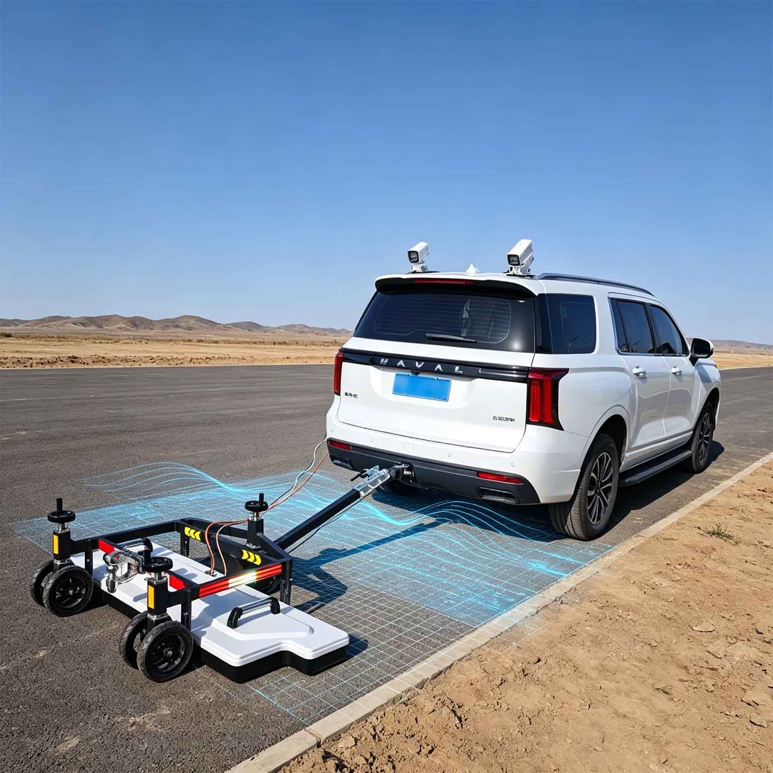
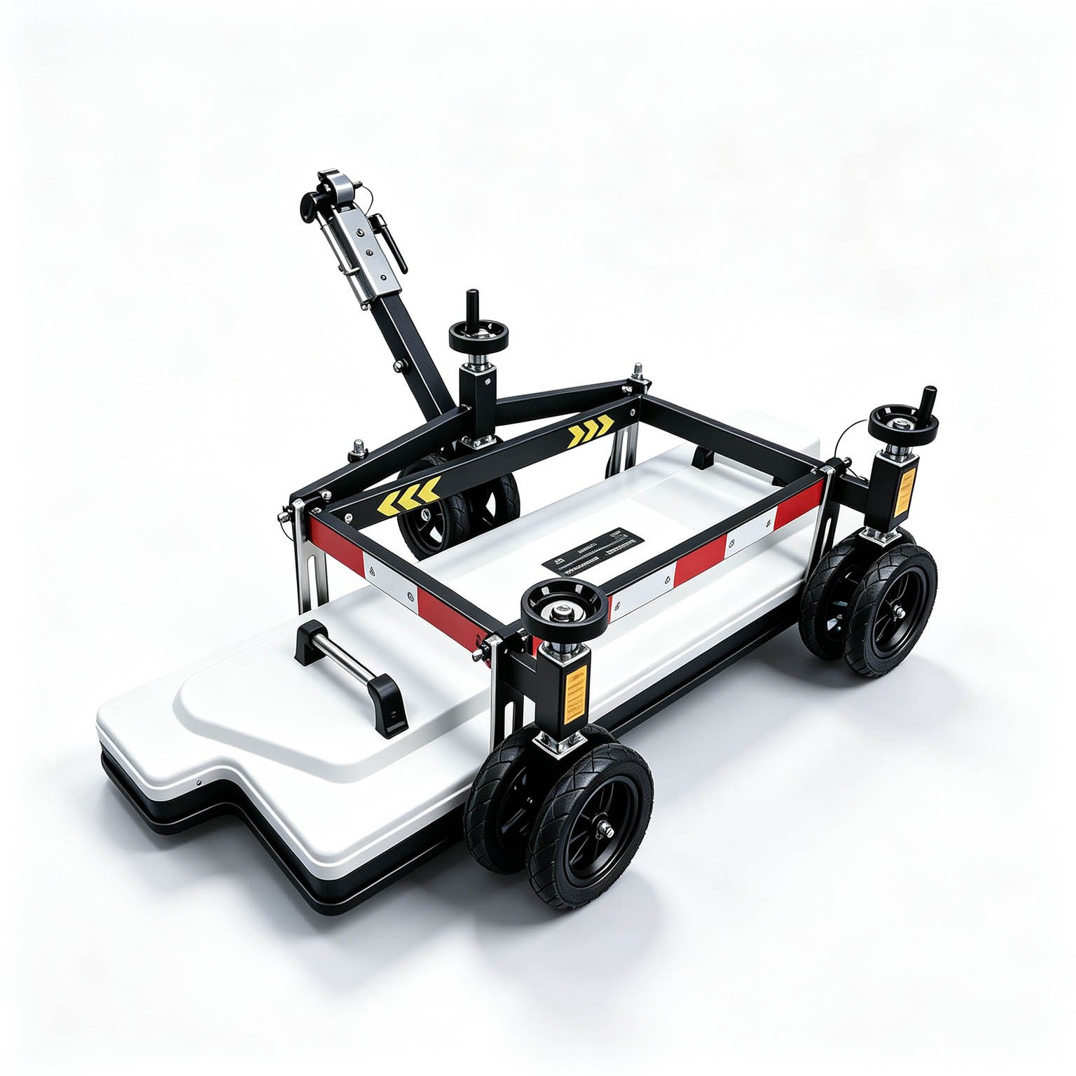
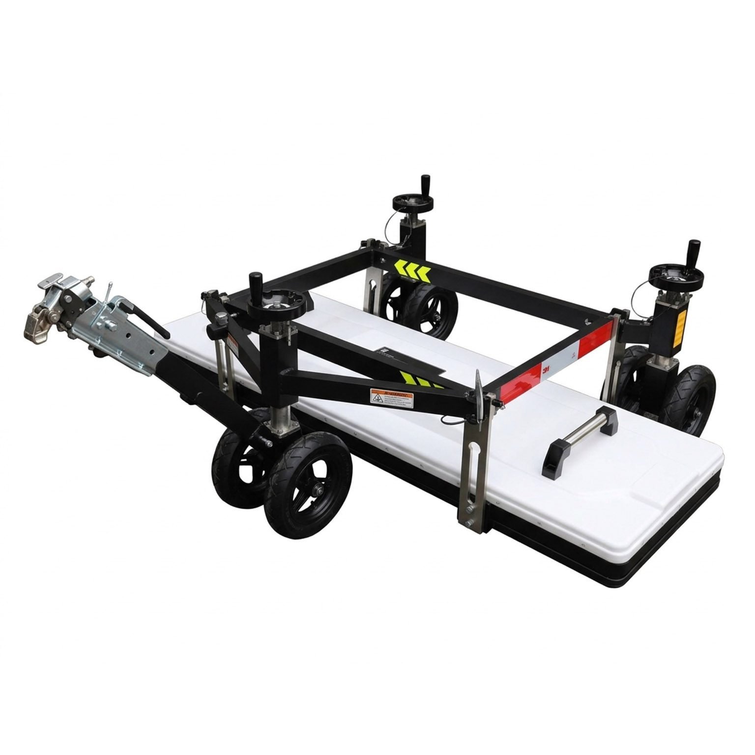
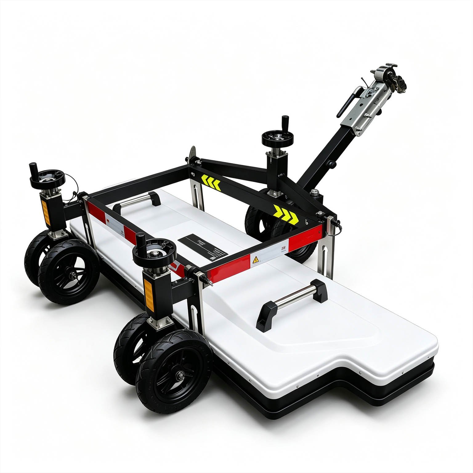
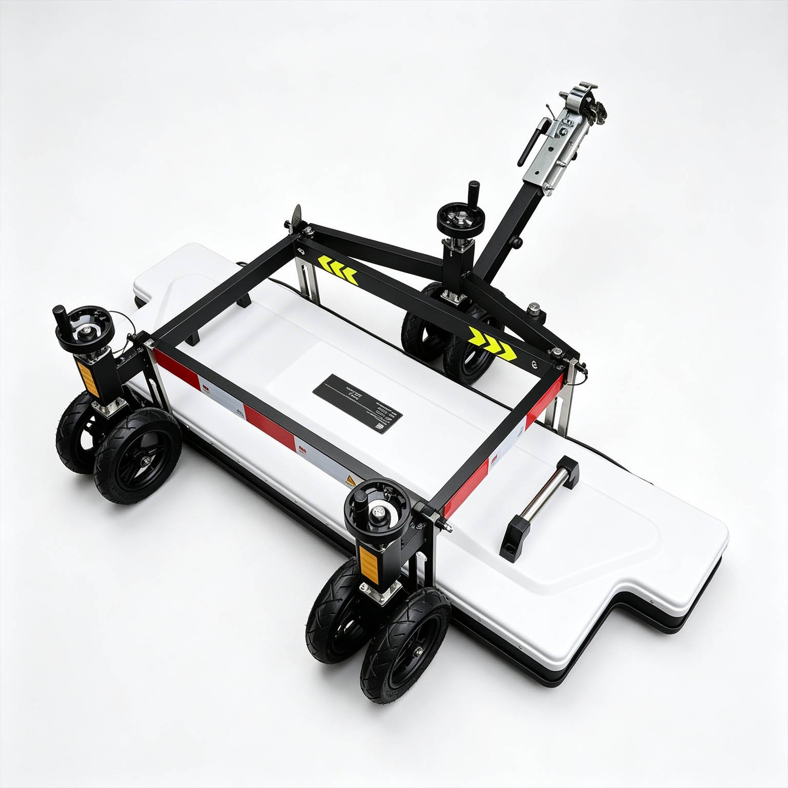
The GEO-GPR-3D-V is a vehicle-mounted 3D ground penetrating radar array built for area coverage rather than single lines. Its 1.8 m-wide antenna carries up to 32 channels at 5.8 cm element pitch — roughly three times the lateral sampling density of comparable deep ground-coupled 3D arrays — and travels on a standard vehicle or inspection truck instead of a towed trailer.
Because transmit and receive elements are freely combinable, the same pass can gather multi-offset data rather than one fixed geometry. That gives the offset families needed for velocity analysis, common-midpoint processing and traveltime tomography, so the 3D model is constrained by measured wave speed rather than by an assumed one.
Technical Highlights
- Three times the lateral density in a wider swath. At 1.8 m and 32 channels the element pitch is 5.8 cm. Where competing deep 3D arrays sample a cross-section at 16.5 cm, this array resolves narrow targets and adjacent services that a coarser grid averages away.
- TX/RX pairs you define. Free combination of transmitting and receiving elements supports multi-offset, CMP and CAP geometries in one deployment, which is what makes velocity analysis and tomographic imaging possible in the field.
- One lane-width pass, fewer overlaps. A 1.8 m swath covers a 3.75 m traffic lane in three passes with 20 per cent overlap, against four passes for a 1.4 m array — a direct saving in lane-closure time on network-level programmes.
- Absolute positioning for volumetric deliverables. RTK with BeiDou and GPS support anchors every trace to a coordinate, so the output is a georeferenced volume — depth slices, plan-view anomaly maps and isosurfaces tied to chainage — not an unregistered section.
Features
- 8 to 64 selectable channels, paired with 0–1.4 m swath width
- Ultra-wideband imaging for high-resolution reflection detail
- One-click configuration with automatic acquisition parameter setting
- RTK positioning with BeiDou and GPS support for coordinate-locked 3D models
- Push-type frame, 1320 × 520 × 180 mm, 16 kg unloaded / 29 kg total
- Works on surfaces where towed and vehicle-mounted arrays cannot be deployed
- Pseudo-colour, stacked-waveform and grayscale display with 3D visualisation
- Pavement layer and thickness identification across the surveyed swath
- Multi-polarisation configurations available on request
Survey Output
What the 3D array actually delivers on a road job:
- Along-line and cross-line sections for layer boundaries and defect depth
- Depth-sliced plan maps (PPI / C-scan) showing voids and services in plan position against chainage
- Isometric volumes for presenting anomaly shape and extent to non-specialists
- Velocity-derived thickness from multi-offset data, without coring for calibration
- Georeferenced anomaly register ready for asset systems and repair scheduling
Applications

| Application | Why the vehicle-mounted array is the right tool |
| Network-level road condition survey | Wide swath and vehicle speed make hundreds of lane-kilometres per campaign practical |
| Municipal utility corridor mapping | 5.8 cm lateral pitch separates adjacent services in congested verges |
| Pavement layer thickness at scale | Multi-offset velocity analysis converts travel time to thickness without coring |
| Subsurface voids and settlement risk | Plan-view depth slices localise cavities to lane position and chainage |
| Airfield apron and runway survey | Continuous coverage with the geometry and positioning an airport audit demands |
| Structural and defect investigation | Multi-polarisation response distinguishes bar-like from layer-like targets |
Depth is set by the working frequency selected and by ground conductivity. The frequency-versus-depth chart is issued with the configuration proposal, so the antenna band matches the target depth of your programme rather than a nominal maximum.
Configuration Guidance
Lateral sampling is the product of channel count and swath width, and it must be set against the smallest target you need to find.
| Channels | Lateral pitch at 1.8 m | Recommended use |
| 32 | ≈5.8 cm | Full 3D void, service and layer survey at dense sampling |
| 16 | ≈12.0 cm | Layer thickness and larger anomalies |
| 8 | ≈25.7 cm | Regional stratigraphy only — select a reduced swath for target work |
For the highest-frequency band on high-permittivity ground (concrete and sound limestone), 34 or more elements across 1.8 m keep the array below its spatial Nyquist limit; specify expected permittivity with your enquiry.
Specifications
| Parameter | Specification |
| Instrument type | Vehicle-mounted multi-channel 3D GPR array |
| Imaging method | Ultra-wideband, freely combinable TX/RX element geometry |
| Channels | 8 / 16 / 32, selected with swath width |
| Coverage width | up to 1.8 m per pass |
| Lateral element pitch | ≈5.8 cm at 32 channels |
| Polarisation | HH standard; multi-polarisation configurable |
| TX/RX configuration | free element pairing supporting multi-offset, CMP and CAP acquisition |
| A/D conversion | 18 bit |
| Signal-to-noise ratio | better than 160 dB |
| Positioning | RTK, BeiDou and GPS support |
| Operation | wired and wireless modes |
| 3D output | three-direction sections, depth slices, plan maps, isosurfaces |
Antenna frequency band, maximum survey speed, along-line trace interval, array mass, envelope dimensions, ingress protection and temperature range are published in the full technical datasheet and are available on request.
FAQ
In gravity exploration (SI), what is the unit of gravity? How to convert gravity units between SI and CGS?
① In SI, it is m·s-2, and one percent of it is the international unit abbreviation g.u.;
② Conversion between SI and CGS: 1g.u.=10-1 mGal
What are gravitational field and gravitational potential?
Gravitational field: The space around the earth with gravity is called the gravitational field.
Gravitational potential: The gravitational potential W in the gravitational field is equal to the work done by a particle of unit mass moving from infinity to that point.
What is the normal gravity field of the earth? What are the rules for the change of the normal gravity field with latitude and altitude?
① The normal gravity field of the earth: Assuming that the earth is a rotating ellipsoid (reference plane), the surface is glossy, the internal density is uniform, or it is distributed in concentric layers, the density of each layer is uniform, and the deviation of the shape of the ellipsoid from the geoid is very small, then the gravity field generated by the earth is the normal gravity field.
② The normal gravity value is only related to the latitude, the smallest at the equator and the largest at the poles, with a difference of about 50,000 g.u.; the rate of change of the normal gravity value with latitude is the largest at 45° latitude, and zero at the equator and the poles; the normal gravity value decreases with increasing altitude, and its rate of change is -3.086 g.u.. The main feature of the long-term change is the "westward drift" of the geomagnetic elements, both the dipole field and the non-dipole field drift westward, and have a global nature.
What is the relationship between gravitational field strength and gravitational acceleration?
The gravitational field strength is equal to the gravitational acceleration in both numerical and dimensional terms, and the two are in the same direction. In gravity exploration, all references to gravity refer to gravitational acceleration. The gravitational field strength at a point in space is equal to the gravitational acceleration at that point.
What is gravity exploration?
Gravity exploration is an exploration method that is based on the density difference of rocks and ores. Since density difference will cause local changes in the normal gravity field of the earth (i.e. gravity anomaly), it is used to solve geological problems by observing and studying gravity anomalies.