What is 2D/3D ERT Survey?

TIPS：This guide helps exploration managers choose between 2D and 3D ERT survey configurations for their specific projects. We explain how advanced resistivity acquisition reduces exploration risk when paired with modern imaging systems. Field engineers and procurement teams will find decision frameworks, deployment workflows, and ROI calculations for subsurface resistivity mapping.

Ⅰ. Introduction

Electrical resistivity tomography has evolved from a niche geophysical method into a standard exploration tool. Early systems used four fixed electrodes and manual switching. A single vertical electrical sounding could take hours. Data density was sparse. Interpretation relied on simplified layer models.

Modern acquisition systems have transformed this landscape. Multi-electrode cables with automated switching collect thousands of data points per hour. Advanced inversion algorithms generate 2D profiles and 3D volumes in minutes. Resolution has improved by orders of magnitude.

The key question for project managers is not whether to use ERT. It is which 2D 3D ERT survey configuration delivers the best results for their budget and timeline. 2D profiling works well for linear targets. 3D volumes are essential for complex geometries. Choosing wrong wastes money and misses targets.

This article provides a practical framework for making this choice. We compare acquisition modes. We detail field deployment procedures. We examine data processing workflows. We also present a real-world case that demonstrates the economic value of selecting the right approach.

Water scarcity affects over two billion people globally. Agriculture consumes approximately 70 percent of freshwater withdrawals. Industry and domestic use compete for the remaining supply. Climate change intensifies these pressures. Droughts become more frequent and severe. Aquifers deplete faster than natural recharge can replenish them.

Sustainable groundwater management requires accurate resource assessment. Managers must know where aquifers exist. They must estimate yield potential. They must understand recharge mechanisms. Geophysical surveys provide this information cost-effectively.

---

Ⅱ. 2D ERT Survey: Linear Profiling for Infrastructure

1. Acquisition Principles

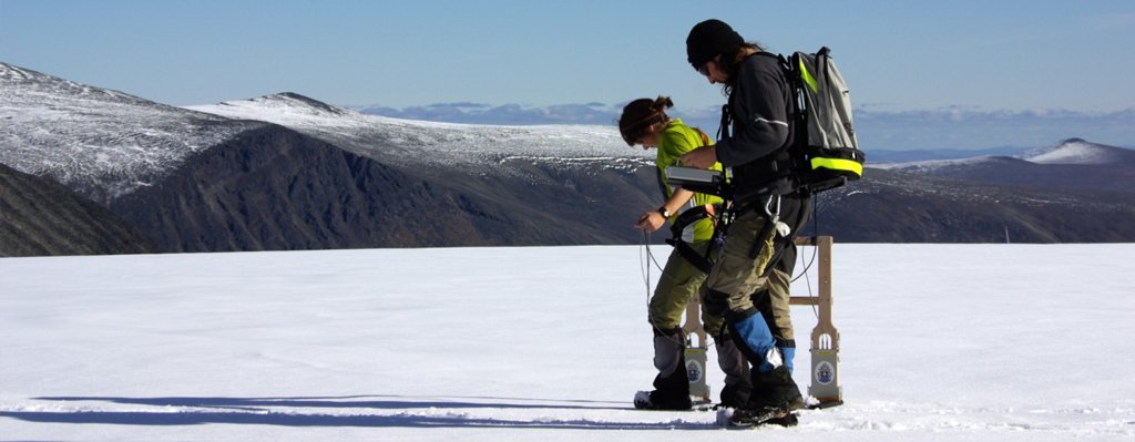
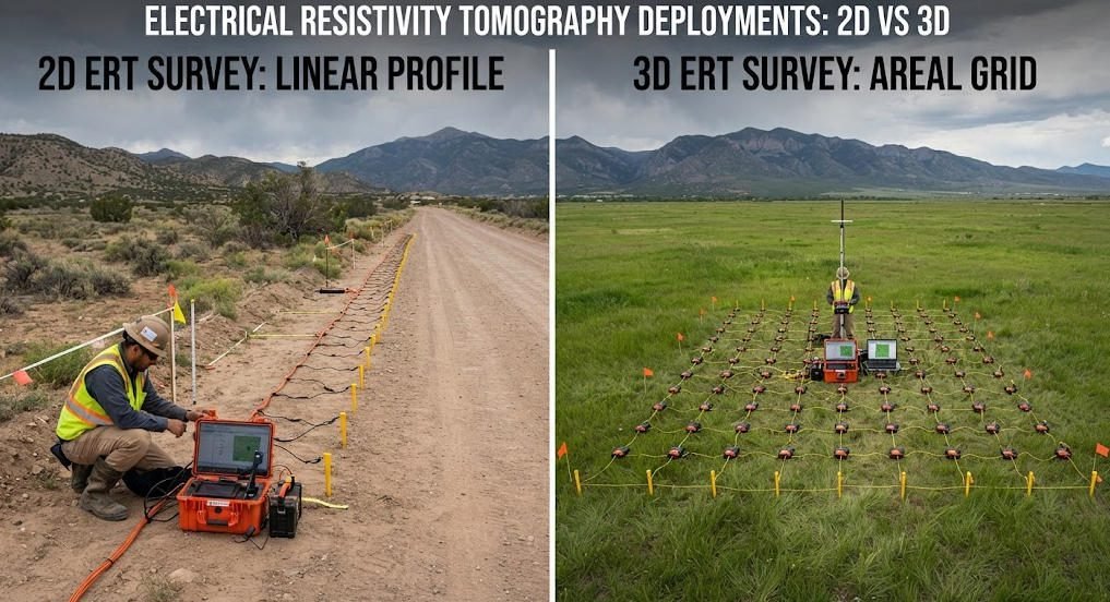
A 2D ERT survey places electrodes along a single line. The instrument auto-selects current and potential electrode pairs. It collects apparent resistivity data for multiple combinations. Inversion software converts these data into a vertical cross-section beneath the profile.

This approach excels for linear infrastructure projects. Road and railway surveys need continuous subsurface imaging along the route. Pipeline integrity assessments require corridor-scale mapping. Dam and levee investigations benefit from cross-sectional views of internal structure.

Standard electrode spacing ranges from 2 to 10 meters. A 120-electrode cable with 5-meter spacing covers 595 meters of profile length. The system collects approximately 3,500 data points per profile. Acquisition time is 30 to 60 minutes for a single profile.

2. Array Selection

Array selection affects image quality significantly. The Wenner array provides excellent vertical resolution. It is ideal for mapping horizontal layers. The dipole-dipole array offers superior lateral resolution. It detects steeply dipping fractures and vertical contacts. The Schlumberger array balances both parameters.

Modern instruments support hybrid arrays. They automatically switch between configurations during acquisition. This flexibility optimizes data quality without extending field time. Crews do not need to re-deploy electrodes for different arrays.

Depth of investigation follows a simple rule. Reliable imaging extends to approximately one-fifth of the total array length. A 600-meter array reaches 120 meters depth. For deeper targets, longer cables or higher power transmitters are needed.

3. Limitations and Cost

2D profiling has limitations. It assumes that geology does not change perpendicular to the profile. Real structures often have complex 3D geometries. A 2D profile through a dipping ore body may misrepresent its true shape. Interpreters must recognize these ambiguities.

Cost efficiency makes 2D ERT survey attractive for reconnaissance work. A typical 2D profile costs $3,000 to $8,000 per kilometer. This investment covers large areas quickly. It identifies targets for detailed 3D follow-up.

---

Ⅲ. 3D ERT Survey: Volumetric Imaging for Complex Targets

1. Grid Acquisition

A 3D ERT survey extends imaging into the subsurface volume. It uses multiple parallel profiles or grid electrode layouts. The instrument measures all possible electrode combinations across the grid. Inversion produces a resistivity cube rather than a cross-section.

This approach is essential for complex targets. Karst terrain contains irregular cavities that 2D profiles cannot resolve. Mine planning requires volumetric models of ore bodies and waste zones. Contaminated sites need detailed plume mapping in all directions. Archaeological surveys search for discrete buried structures.

Grid electrode layouts provide the highest data density. Electrodes are placed in a rectangular grid pattern. Spacing typically ranges from 2 to 20 meters. A 20-by-20 grid with 5-meter spacing uses 400 electrodes. The system collects hundreds of thousands of data points.

2. Cable Management and Wireless Nodes

Cable management becomes the main logistical challenge. Traditional systems use multi-core cables that connect every electrode to the central unit. These cables are heavy and bulky. A 400-electrode survey may require several kilometers of cable. Field crews spend significant time on cable deployment.

Wireless electrode nodes solve this problem. Each node contains its own acquisition circuit and battery. Nodes communicate with a central controller via radio or Bluetooth. This eliminates heavy cables entirely. Deployment speed increases by a factor of five to ten.

3. Inversion and Resolution

3D inversion demands substantially more computing power than 2D processing. A typical 3D dataset contains 100,000 to 1,000,000 data points. Inversion meshes may have 500,000 to 2,000,000 cells. Processing time ranges from hours to days depending on hardware.

Cloud computing has changed this equation. Field crews upload raw data to remote servers. High-performance clusters run inversion algorithms in parallel. Results return within hours. This workflow eliminates the need for powerful local workstations.

High density resistivity imaging in 3D mode delivers resolution that was impossible a decade ago. Modern systems achieve 0.2-meter voxel resolution in favorable conditions. This precision enables detection of small targets like buried pipes or thin mineral veins.

---

Ⅳ. Decision Matrix: When to Choose 2D vs 3D

1. Linear Infrastructure

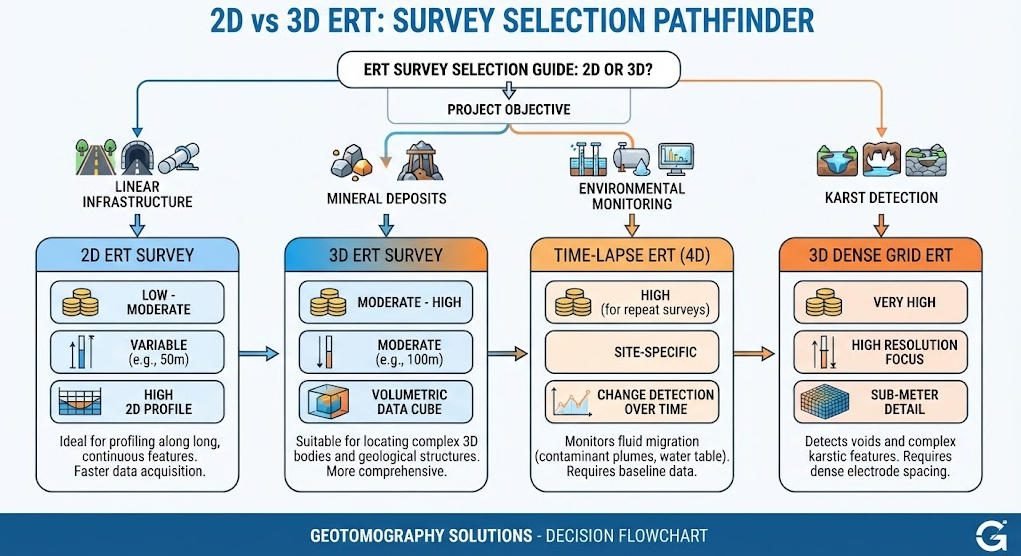
For linear infrastructure such as roads, pipelines, and tunnels, use 2D profiling. Deploy electrodes along the project corridor. Use Wenner or hybrid arrays for balanced resolution. Budget $3,000 to $8,000 per kilometer of profile.

2. Mineral Deposits

For complex mineral deposits such as disseminated ore bodies and vein systems, use 3D grids. Deploy electrodes in a rectangular pattern covering the target area. Use dipole-dipole or gradient arrays for lateral resolution. Budget $15,000 to $50,000 per square kilometer.

3. Environmental Monitoring

For environmental monitoring such as contaminant plumes and landfill integrity, use time-lapse 2D or 3D surveys. Repeat surveys track changes over time. Differential imaging highlights active processes. Budget depends on monitoring frequency.

4. Karst and Cavities

For karst and cavity detection, use 3D grids with closely spaced electrodes. Cavity walls create sharp resistivity contrasts. High spatial resolution is essential for reliable detection. Budget $20,000 to $60,000 per square kilometer.

---

Ⅴ. Field Deployment Workflow

1. Site Reconnaissance

Field deployment follows a systematic workflow. Step one is site reconnaissance. Crews assess terrain, access, and cultural noise sources. They identify optimal profile or grid locations. They also check for buried utilities and overhead power lines.

2. Electrode Placement

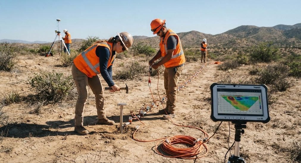
Step two is electrode placement. For 2D surveys, crews lay out the cable along the profile line. They insert electrodes at regular intervals. Contact resistance must remain below 10 kilo-ohms. Dry soils require saltwater or bentonite gel around electrodes.

For 3D surveys, crews place electrodes in a grid pattern. They use GPS or total stations for precise positioning. Position errors must stay within 10 percent of electrode spacing. Larger errors degrade inversion accuracy.

3. System Configuration

Step three is system configuration. Operators program the instrument with array type, electrode spacing, and measurement schedule. They test a few electrode pairs to verify contact quality. They also check for noise levels across the frequency spectrum.

4. Data Acquisition

Step four is data acquisition. The instrument auto-cycles through electrode combinations. Real-time quality monitoring displays apparent resistivity values. Operators watch for outliers that indicate bad contacts or noise spikes. They pause acquisition to fix problems immediately.

5. Data Validation

Step five is data validation. Crews review pseudosections for coherent patterns. Random scatter indicates noise or poor contacts. Systematic trends suggest real geology. They also compare adjacent profiles for consistency.

---

Ⅵ. Data Processing and Inversion

1. Data Cleaning

Data processing begins with data cleaning. Operators remove noisy data points. They correct for topographic effects. They also normalize for array geometry factors. Clean data improves inversion convergence and result reliability.

2. Inversion Algorithms

Inversion transforms apparent resistivity data into true resistivity models. The algorithm minimizes the difference between observed and calculated data. It also applies regularization constraints to produce geologically plausible models.

Smoothness-constrained inversion is the standard approach. It penalizes rough models while fitting the data. This approach works well for gradational geological boundaries. Sharp boundary inversion preserves discrete contacts. It is better for fault zones and cavity walls.

Modern systems incorporate AI-powered adaptive inversion. Machine learning algorithms analyze data characteristics. They automatically select optimal inversion parameters. This reduces the need for manual parameter tuning. It also improves result consistency across different datasets.

3. Interpretation

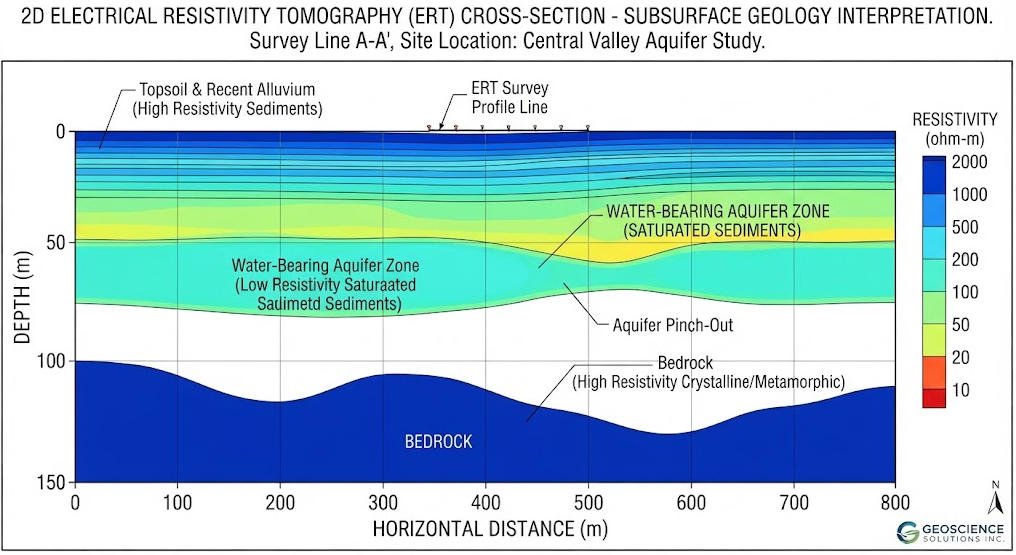
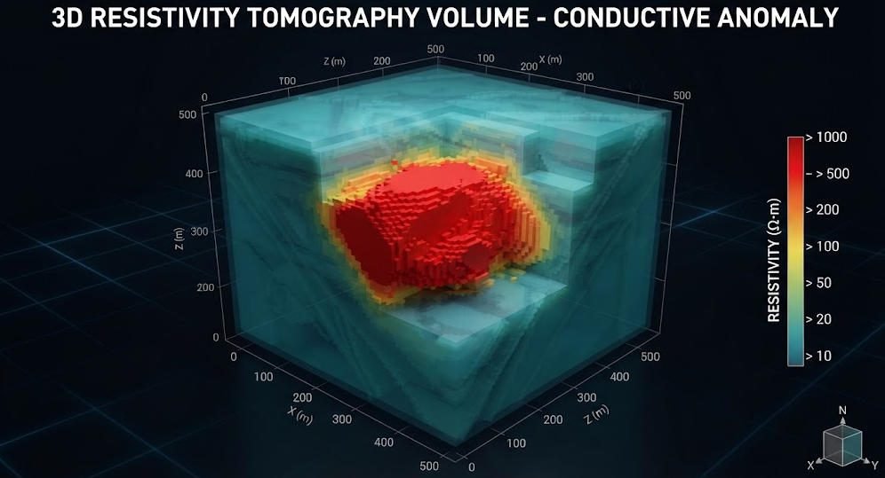
Interpretation focuses on identifying resistivity anomalies. Low-resistivity zones may indicate water, clay, or mineralization. High-resistivity zones may indicate fresh rock, voids, or dry sediments. Borehole calibration reduces ambiguity.

4. Case Study: Lithium Exploration

A recent lithium exploration project demonstrated the value of 3D ERT. The target was spodumene-bearing pegmatite dikes in structurally complex terrain. Previous 2D 3D ERT survey attempts using conventional methods missed narrow veins.

The project team deployed a high density resistivity imaging system across 25 square kilometers. They used a hybrid dipole-gradient array configuration. Electrode spacing was 20 meters. The grid contained 625 electrodes.

Acquisition completed in 12 days. The system collected over 1 million data points. AI-powered inversion processed the dataset in 18 hours. The resulting 3D model revealed a network of thin conductive dikes.

Drilling targeted the anomalies identified in the resistivity model. Success rate improved from 51 to 93 percent. The minimum detectable vein size was 0.5 by 0.3 by 0.2 meters. This resolution was 160 times better than conventional methods.

Total exploration cost dropped by 69 percent. The 3D survey cost was significantly lower than conventional grid drilling. The savings funded additional exploration in adjacent blocks.

This case illustrates several key principles. First, 3D imaging is essential for complex vein systems. 2D profiles would have missed most targets. Second, high channel counts and dense electrode spacing improve resolution dramatically. Third, AI inversion reduces processing time from weeks to hours.

---

Ⅶ. Technical Factors and Equipment Selection

1. Contact Quality and Noise

Several technical factors affect survey success. Electrode contact quality is critical. Poor contact injects noise and reduces signal strength. Crews must monitor contact resistance throughout acquisition.

Cultural noise from power lines and pipelines degrades data quality. Surveys near infrastructure require careful planning. Remote reference techniques or time-domain filtering may be needed.

Topography affects current flow patterns. Hills and valleys distort the electric field. Software corrections account for surface elevation changes. Accurate topographic surveys are essential for reliable inversion.

Seasonal variations change near-surface resistivity. Wet seasons lower resistivity in the topsoil. Dry seasons increase it. Time-lapse surveys must account for these changes when interpreting temporal differences.

2. Hardware Specifications

Equipment selection depends on project requirements. Channel count determines survey speed. More channels collect data faster. A 256-channel system completes a large 3D survey in days. A 64-channel system may need weeks.

Power output determines depth penetration. High-power transmitters inject more current. They overcome contact resistance and reach deeper targets. Deep mineral exploration needs 5,000 to 10,000 watt transmitters.

Temperature range affects field reliability. Extreme environments demand rugged hardware. Systems rated for minus 40 to plus 85 degrees Celsius handle most conditions. Specialized units operate in polar or desert extremes.

Equipment portability has improved dramatically. Early resistivity meters weighed over 50 kilograms. They required vehicle transport and generator power. Modern systems fit in a single backpack. Battery packs provide 12 hours of continuous operation. This portability enables surveys in remote terrain where vehicle access is impossible.

Data visualization has also evolved. Early interpreters relied on printed pseudosections and contour maps. Modern software displays 2D profiles and 3D volumes on tablets in the field. Real-time color maps let crews adjust layouts before leaving the site. This immediate feedback reduces costly return visits.

Quality assurance protocols ensure reliable results. Pre-survey tests verify instrument calibration. Post-survey checks confirm data completeness. Intermediate tests monitor electrode contact throughout acquisition. These steps catch problems early. They prevent the discovery of bad data back in the office.

Training requirements have decreased with modern interfaces. Touchscreen menus guide operators through setup. Automated wizards suggest optimal parameters for common targets. Novice users can collect reliable data after a few days of training. However, complex interpretations still require experienced geophysicists.

3. Future Trends

The future of resistivity imaging points toward autonomous systems. Permanent electrode arrays enable continuous monitoring. Wireless nodes transmit data to central servers. AI algorithms detect anomalies in real time.

These innovations will transform environmental monitoring. Leak detection from storage tanks and pipelines will trigger immediate alerts. Mine tailings dam integrity will be tracked continuously. Groundwater resources will be managed with unprecedented precision.

For exploration teams, the message is clear. Modern acquisition systems deliver results that were impossible a decade ago. The choice between 2D and 3D is no longer a technical luxury. It is a strategic decision that determines project success.

Reference Sources

Name	URL
U.S. Geological Survey — Electrical Resistivity Tomography Data Catalog	https://catalog.data.gov/?q=electrical+resistivity+tomography
MDPI Geosciences — Optimized Arrays for 2-D Resistivity Survey Lines	https://www.mdpi.com/2076-3263/16/5/182
MDPI Minerals — ERT with Archie’s Law for Rare Earth Deposit Characterization	https://www.mdpi.com/journal/minerals?cid=42575
CLU-IN — Electrical Resistivity Tomography Case Studies	https://clu-in.org/characterization/technologies/default2.focus/sec/Geophysical_Methods/cat/Electrical_Resistivity_Tomography/
Britannica — Electrical and Electromagnetic Methods in Earth Exploration	https://www.britannica.com/topic/Earth-exploration/Electrical-and-electromagnetic-methods

---

FAQ