How to Calibrate a Magnetometer Properly？丨Magnetometer Calibration

TIPS：Magnetometer calibration ensures every proton magnetometer delivers reliable field data. This guide explains the complete magnetometer calibration process using IGRF reference standards and Helmholtz coil verification. You will learn how proton magnetometer calibration eliminates drift errors and why regular magnetometer calibration remains essential for accurate geophysical survey results.

Ⅰ. Why Magnetometer Calibration Matters

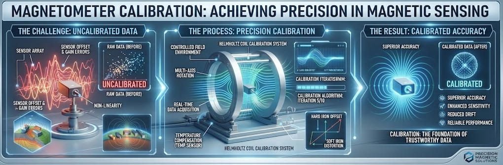
Every magnetometer drifts over time. Sensors age. Electronics shift. Environmental factors alter performance. Regular magnetometer calibration corrects these changes before they corrupt survey data.

1. The Cost of Uncalibrated Instruments

Uncalibrated magnetometers hide errors within measurements. A 5-nanotesla offset seems small. Over a 50-kilometer survey line, this error accumulates. Anomaly shapes distort. Target depths mislead interpreters.

Mineral exploration projects suffer most. Weak magnetic signatures disappear into noise. Ore bodies remain undiscovered. Companies waste drilling budgets on false targets. Proper magnetometer calibration prevents these losses.

2. Traceability to International Standards

Geophysical surveys must connect to global reference systems. The International Geomagnetic Reference Field (IGRF) provides this link. Calibrated instruments align with this model. Results become comparable across projects and decades.

National observatories maintain absolute standards. Their measurements anchor the IGRF. Field instruments trace accuracy back to these facilities. This chain of traceability validates commercial survey results.

3. Regulatory and Contractual Requirements

Many jurisdictions mandate calibrated instruments. Environmental assessments require documented accuracy. Mining permits specify measurement standards. Academic publications demand calibration certificates.

Clients increasingly request calibration documentation. Insurance companies review survey quality. Legal disputes hinge on measurement reliability. Magnetometer calibration protects professional reputations.

Ⅱ. Understanding Proton Magnetometer Calibration Principles

Proton magnetometers measure absolute field strength. They do not require vector orientation. This simplifies calibration compared to fluxgate devices. However, specific procedures ensure optimal performance.

1. How Proton Precession Creates Measurable Signals

Hydrogen-rich fluids contain protons with magnetic moments. A polarizing current aligns these moments. After polarization stops, protons precess around Earth’s field. The precession frequency equals the Larmor constant times field strength.

Oscillators count this frequency. Stable oscillators yield accurate counts. Temperature drift in the oscillator creates proportional field errors. Proton magnetometer calibration verifies oscillator stability against known references.

2. Sources of Measurement Error

Several factors affect proton magnetometer accuracy. Oscillator drift remains primary. Temperature changes alter crystal frequency. Aging components shift electrical characteristics.

Sensor orientation affects signal amplitude. Tilted sensors capture smaller precession signals. Low signal-to-noise ratios increase counting uncertainty. Proper alignment during calibration ensures optimal geometry.

Polarizing current strength influences signal quality. Weak polarization leaves protons partially aligned. Strong currents may heat the sensor fluid. Optimal current levels balance signal strength against thermal effects.

3. The Role of Reference Standards

Calibration requires known magnetic fields. Several sources provide these references. Geomagnetic observatories publish absolute measurements. The IGRF model predicts field values globally. Helmholtz coils generate controlled artificial fields.

Observatory comparisons offer highest accuracy. Field teams visit established stations. They compare instrument readings against observatory values. Differences reveal instrument offsets.

IGRF models suit remote locations. Software calculates expected field strength at any coordinate. Comparisons against this model identify drift. Model accuracy of approximately 10 nanotesla suffices for most applications.

Helmholtz coils enable laboratory calibration. These devices create uniform magnetic fields. Known currents produce calculable field strengths. Coil dimensions determine uniformity volumes. Proton magnetometers fit within these volumes for precise adjustment.

Ⅲ. Step-by-Step Magnetometer Calibration Process

Systematic procedures ensure consistent results. This section details each calibration stage.

1. Pre-Calibration Inspection and Preparation

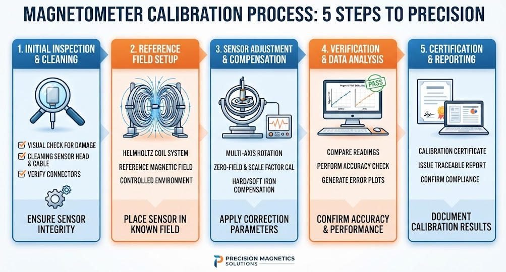
Begin with visual inspection. Check sensor housing for cracks. Examine cables for wear. Verify connector integrity. Physical damage often causes subtle errors.

Test battery voltage under load. Weak batteries affect polarizing current. Reduced current degrades signal quality. Replace batteries showing voltage drop during polarization cycles.

Clean all magnetic contaminants. Remove watches and jewelry. Keep mobile phones distant. Survey vehicles may affect readings. Establish calibration zones at least 50 meters from vehicles.

Allow temperature stabilization. Instruments transported in air-conditioned vehicles need acclimation. Thirty minutes typically suffices. Sudden temperature changes affect oscillator stability.

2. Reference Field Establishment

Select a magnetically quiet location. Avoid power lines and buried pipes. Test for cultural interference using multiple readings. Stable values indicate suitable sites.

Record geographic coordinates precisely. GPS accuracy affects IGRF comparisons. Use differential GPS when available. Document elevation above sea level.

Measure the field over extended periods. Ten-minute observations reveal diurnal trends. Compare averages against IGRF predictions. Note differences for correction application.

3. Sensor Adjustment and Axis Alignment

Position the sensor vertically. The precession signal maximizes when the sensor axis aligns with Earth’s field. Use inclinometers for precise alignment. Typical dip angles range from 30 to 90 degrees depending on latitude.

Rotate the sensor around its vertical axis. Measurements should remain constant for scalar instruments. Variations indicate cross-axis sensitivity. Document any azimuth dependence.

Apply correction factors through instrument software. Scale factors adjust sensitivity. Offset values correct baseline drift. Tilt compensations account for non-vertical deployment.

4. Multi-Point Verification

Validate calibration across field ranges. Measure at locations with different field strengths. High-latitude sites show stronger fields. Equatorial regions display weaker values. Confirm linear response throughout the operational range.

Test gradient tolerance if applicable. Place sensors at known separations. Measure gradient between positions. Compare against calculated values. Gradient errors indicate sensor matching problems.

5. Documentation and Certification

Record all calibration parameters. Note reference values used. Document environmental conditions. Include temperature and time of day. These details support future troubleshooting.

Generate calibration certificates. List instrument serial numbers. Specify correction factors applied. Include reference traceability statements. Signed certificates satisfy client requirements.

Archive calibration histories. Track drift trends over time. Identify instruments needing more frequent adjustment. Historical data guides maintenance scheduling.

Ⅳ. IGRF and Observatory Standards for Magnetometer Calibration

International standards anchor calibration procedures. Understanding these references improves calibration quality.

1. The International Geomagnetic Reference Field (IGRF)

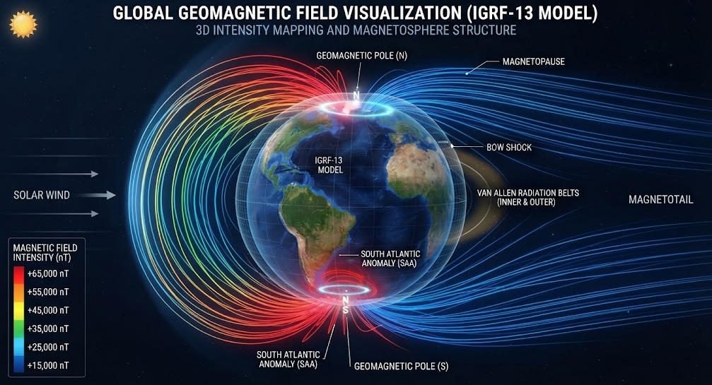
The IGRF models Earth’s main magnetic field. International associations update coefficients every five years. The model includes spherical harmonic expansions to degree 13. This resolution captures global field variations.

Field values calculated from IGRF serve as calibration references. Accuracy typically reaches 10 nanotesla during quiet conditions. Solar storms increase uncertainty. Calibrate during magnetically quiet periods for best results.

Software tools simplify IGRF calculations. Enter coordinates and elevation. Select appropriate model epoch. The program outputs expected field components. Total intensity values suit scalar proton magnetometer comparisons.

2. Geomagnetic Observatory Networks

Global observatories provide absolute measurements. INTERMAGNET coordinates these facilities. Over 150 observatories contribute data. Standards ensure consistency across stations.

Observatories use specialized instruments. Proton magnetometers measure total intensity. Fluxgate theodolites determine declination and inclination. Absolute measurements anchor regional field models.

Field calibration against observatories offers highest accuracy. Teams transport instruments to nearby stations. Simultaneous measurements reveal instrument offsets. This direct comparison eliminates model uncertainties.

3. Helmholtz Coil Systems for Laboratory Calibration

Helmholtz coils generate uniform magnetic fields. Two coaxial circular coils create central uniformity. Coil spacing equals coil radius for standard configurations. Field strength depends on current and geometry.

Laboratory calibration proceeds systematically. Place the proton magnetometer at the coil center. Apply known currents. Measure resulting fields. Compare instrument readings against calculated values.

Multi-axis coil systems enable vector calibration. Three orthogonal coil pairs create arbitrary field directions. This capability suits fluxgate magnetometer calibration. Scalar proton magnetometers require only total field verification.

4. Calibration Transfer Standards

Transfer standards bridge laboratory and field environments. Portable reference magnetometers travel to survey sites. These instruments maintain calibration through infrequent observatory comparisons.

Survey instruments compare against transfer standards. Differences indicate field instrument drift. This approach avoids transporting delicate laboratory equipment. It brings traceability directly to project locations.

Ⅴ. Calibration Frequency Guidelines

Optimal calibration intervals balance accuracy against logistics. Several factors influence scheduling decisions.

1. Deployment Intensity

Daily field use accelerates drift. Vibration affects sensor alignment. Temperature cycling stresses electronics. Frequent calibration catches problems early.

Weekly calibration suits intensive programs. Daily mineral exploration surveys demand this frequency. Archaeological grids with tight schedules benefit similarly. Short intervals prevent error accumulation.

2. Environmental Severity

Harsh environments stress instruments. Desert heat expands components. Arctic cold contracts seals. Humidity corrodes connectors. Each factor accelerates drift.

Every three to five days suits extreme conditions. Offshore surveys face salt spray. Tropical projects endure monsoon humidity. Mountain surveys encounter rapid weather changes. Shorten intervals when conditions challenge instrument stability.

3. Storage and Transportation

Long storage periods affect calibration. Batteries may leak. Capacitors degrade. Mechanical shock during transport shifts alignment.

Calibrate after extended storage. Three months idle warrants fresh verification. Post-repair calibration remains mandatory. Any disassembly requires recertification.

4. Instrument Age and History

New instruments stabilize during initial use. Components settle into equilibrium. Early calibration establishes baselines. Subsequent intervals may lengthen as instruments mature.

Aging instruments need closer monitoring. Oscillator crystals drift faster with age. Sensor fluids may degrade. Historical drift rates guide interval selection. Instruments showing rapid drift need attention.

5. Smart Calibration Features

Modern proton magnetometers include self-checking routines. Internal references verify oscillator stability. Software alerts operators when drift exceeds thresholds. These features supplement but do not replace full calibration.

Auto-calibration modes simplify field procedures. Instruments compare current readings against stored references. Significant deviations trigger warnings. Operators then perform detailed calibration.

Ⅵ. Common Calibration Challenges and Solutions

Even careful procedures encounter problems. Recognizing symptoms speeds resolution.

1. Residual Field Interference

Nearby ferrous objects distort local fields. Steel fences create permanent anomalies. Vehicles produce strong disturbances. Even reinforced concrete affects measurements.

Symptoms include inconsistent repeated readings. Values change with sensor position. Azimuth dependence appears in scalar data. These signs indicate cultural interference.

Solutions require site selection discipline. Test candidate locations with multiple readings. Move suspected interference sources away. Use magnetic shielding when relocation proves impossible.

2. Temperature-Induced Drift

Oscillator frequency changes with temperature. Morning and afternoon readings diverge. Daily patterns repeat consistently. Seasonal variations add long-term trends.

Symptoms show as systematic daily curves. Field values track ambient temperature. Instruments warm up during operation. Readings stabilize after thermal equilibrium.

Solutions include temperature-compensated oscillators. OCXO technology maintains constant crystal temperature. Allow adequate warm-up time before critical measurements. Record temperature for post-survey corrections.

3. Sensor Alignment Errors

Improper tilt reduces signal amplitude. Precession signals weaken below detection thresholds. Counting uncertainty increases. Noisy readings result.

Symptoms include erratic values. Readings vary with sensor orientation. Signal quality indicators show degradation. These signs suggest alignment problems.

Solutions use precision inclinometers. Bubble levels provide rough alignment. Electronic tilt sensors offer better accuracy. Verify verticality before each measurement session.

4. Software and Firmware Issues

Calibration algorithms contain assumptions. Incorrect parameters produce wrong corrections. Firmware bugs affect calculations. Software updates may change behavior.

Symptoms include sudden calibration changes. Post-update readings shift unexpectedly. Manual calculations disagree with instrument outputs. These signs indicate software problems.

Solutions maintain software version records. Verify calculations independently when possible. Contact manufacturers for known issues. Apply patches promptly when available.

5. Battery and Power Supply Problems

Weak batteries affect polarizing current. Reduced current leaves protons partially aligned. Signal strength drops. Counting errors increase.

Symptoms include declining signal quality indicators. Measurements become noisier over time. Instrument shuts down unexpectedly. These signs indicate power problems.

Solutions monitor battery voltage continuously. Replace batteries before critical surveys. Use external power when possible. Carry spare battery packs for extended operations.

Ⅶ. The JPMG Series Calibration Protocol

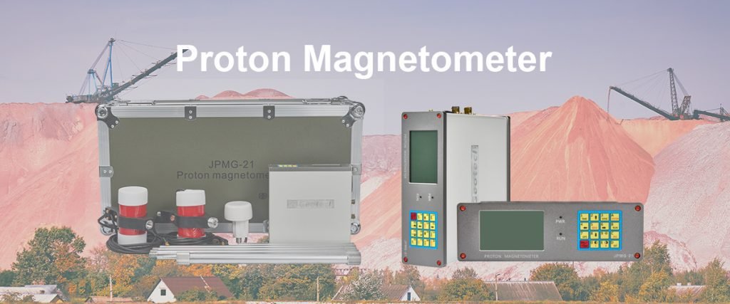
Geotech’s JPMG Series proton magnetometers incorporate advanced calibration features. This section describes their specific protocols.

1. Factory Calibration Standards

Each JPMG instrument undergoes rigorous factory calibration. Helmholtz coil systems verify absolute accuracy. Temperature chambers test oscillator stability. Vibration tables simulate field transport.

Factory certificates document initial performance. Absolute accuracy reaches plus or minus 0.1 nanotesla. Resolution specifications confirm 0.01 nanotesla capability. These values serve as lifetime benchmarks.

2. Field Calibration Procedures

Field calibration follows streamlined procedures. Internal reference oscillators enable self-checks. Operators compare readings against IGRF values. Software guides correction factor application.

GPS integration automates coordinate entry. IGRF calculations occur automatically. Expected values display in real time. Differences guide adjustment decisions.

3. Long-Term Stability Monitoring

JPMG instruments store calibration histories. Drift trends appear graphically. Operators identify gradual degradation. Predictive maintenance prevents sudden failures.

Cloud connectivity enables remote diagnostics. Manufacturer support reviews instrument health. Calibration reminders appear automatically. This proactive approach maximizes uptime.

Ⅷ. Best Practices for Calibration Management

Effective programs require systematic management. These practices ensure consistent quality.

1. Maintain Calibration Schedules

Create calendars for each instrument. Record last calibration dates. Project next required calibration. Alert operators before deadlines pass.

Digital systems automate scheduling. Database entries track instrument histories. Automated emails remind responsible personnel. Integration with project planning prevents conflicts.

2. Document Everything

Calibration records require comprehensive documentation. Instrument serial numbers identify specific units. Environmental conditions explain unusual results. Operator names enable follow-up questions.

Digital logs simplify retrieval. Searchable databases find historical records. Trend analysis identifies problem instruments. Audit trails satisfy quality inspectors.

3. Train Personnel Thoroughly

Calibration requires specific skills. Operators must understand magnetic principles. They need proficiency with instrument software. Recognition of abnormal symptoms prevents bad data.

Training programs combine theory and practice. Classroom sessions cover fundamentals. Hands-on workshops develop skills. Certification tests verify competency.

4. Use Accredited Services When Required

Some projects demand accredited calibration. ISO standards specify traceability requirements. Accredited laboratories meet these standards. Their certificates carry official recognition.

Geotech provides accredited calibration services. National standards laboratories verify our procedures. Clients receive internationally recognized documentation. This service supports highest-quality projects.

Ⅸ. Conclusion

Magnetometer calibration transforms instruments from potential error sources into reliable measurement tools. Proton magnetometer calibration connects field data to international standards. Regular procedures catch drift before it corrupts surveys.

The IGRF provides global reference values. Observatory comparisons offer direct traceability. Helmholtz coils enable laboratory verification. Combined approaches ensure measurement confidence.

Calibration frequency depends on use intensity and environmental severity. Daily deployment warrants weekly checks. Harsh conditions demand shorter intervals. Smart instruments supplement but do not replace formal procedures.

Geotech supports calibration excellence through the JPMG Series. Factory calibration establishes baselines. Field procedures simplify verification. Long-term monitoring prevents surprises. Contact our team for calibration services and training programs.

Accurate geophysical data begins with proper magnetometer calibration. Invest in calibration discipline. Reap rewards in survey quality and professional reputation.

Reference Sources

Organization	URL
INTERMAGNET – International Real-time Magnetic Observatory Network	https://www.intermagnet.org/
International Association of Geomagnetism and Aeronomy (IAGA)	https://www.iaga-aiga.org/
USGS Geomagnetism Program	https://geomag.usgs.gov/
British Geological Survey (BGS) – Geomagnetism	https://www.bgs.ac.uk/geology-projects/geomagnetism/
NOAA National Centers for Environmental Information (NCEI)	https://www.ncei.noaa.gov/products/international-geomagnetic-reference-field

---

Proton Magnetometer | Dual-Sensor Version

---

FAQ