What Are Resistivity Meters? 2026 Complete Technical Guide

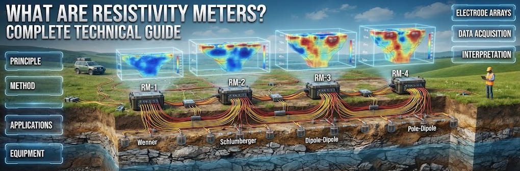
Overview：This technical guide explains how resistivity meters measure subsurface structures through controlled current injection. It covers the physics behind resistivity meter design, compares electrode array configurations, and maps resistivity meter selection criteria for mining, geotechnical and environmental projects.

Ⅰ. Definition and Operating Principles

1. Core Definition

Resistivity meters are geophysical instruments that inject electrical current into the ground and measure resulting voltage to map subsurface resistivity contrasts.

2. Ohm’s Law and Apparent Resistivity

Resistivity measurement derives directly from Ohm’s Law, expressed as V = I × R. The instrument injects a known current I through two current electrodes and measures the voltage V between two potential electrodes. The ratio V/I gives resistance R, which is then converted into apparent resistivity ρa using a geometric factor. Apparent resistivity differs from true resistivity because the ground is never homogeneous. It represents a weighted average of all materials within the volume of current flow. Only through inversion modeling does apparent resistivity become a true subsurface resistivity model.

3. The Four-Electrode Configuration

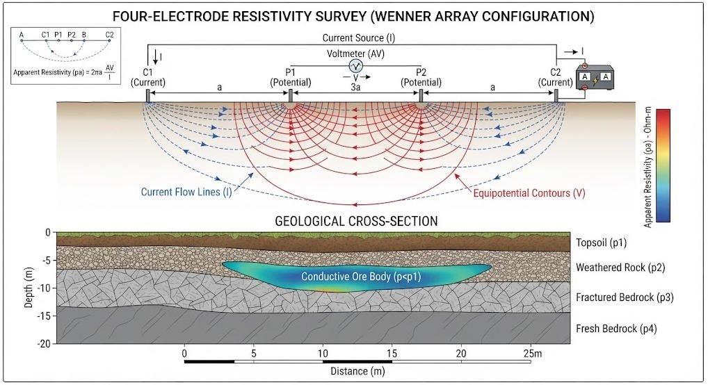
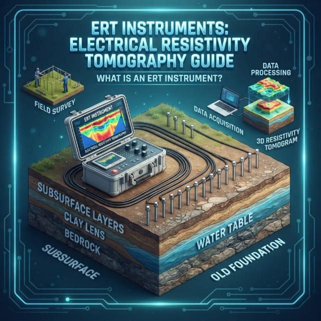
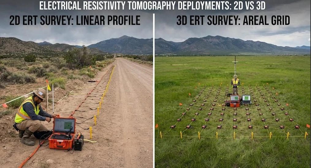
Modern resistivity meters use a minimum of four electrodes in a linear or planar layout. Two outer electrodes inject current, while two inner electrodes measure potential difference. This configuration eliminates the contact resistance error that plagues two-electrode systems. The measured potential is independent of the current electrode contact quality. Standard surveys deploy dozens to hundreds of electrodes with automated switching. This enables 2D profiling and 3D volumetric imaging without manual reconfiguration.

4. Geometric Factor and Array Formulas

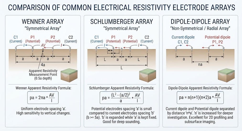
Each electrode arrangement has a characteristic geometric factor K that converts measured resistance into apparent resistivity. The K value depends solely on electrode spacing, not on the ground properties. The following table lists standard formulas for the three most common arrays.

Array Type	Geometric Factor K	Signal Strength	Primary Survey Mode
Wenner	2πa	High	Horizontal profiling
Schlumberger	π(b² − a²)/(4a)	Medium	Vertical sounding
Dipole-Dipole	πn(n+1)(n+2)a	Low	Lateral anomaly mapping

Where a is the potential electrode spacing, b is the current electrode spacing, and n is the dipole separation multiplier. Apparent resistivity is calculated as ρa = K × (V/I) for all array types. Array choice directly controls depth of investigation and spatial resolution.

Ⅱ. Instrument Architecture and Core Components

1. Transmitter Unit

The transmitter generates the controlled DC current that energizes the subsurface. Modern systems output from 100mA to 10A depending on target depth and ground resistance. High-power transmitters deliver 5kW or 10kW for deep mineral surveys. Digital transmitters produce clean square-wave or alternating polarity waveforms. Polarity reversal suppresses self-potential and electrode polarization effects.

2. Receiver and Measurement Chain

The receiver amplifies and digitizes the potential difference between measurement electrodes. Modern receivers use 24-bit analog-to-digital conversion for high measurement precision. This digitization delivers 120dB or higher dynamic range in noisy urban environments. Stacking repeats measurements multiple times to average out random noise. Input impedance above 100MΩ prevents loading errors from high-resistance ground contacts.

3. Electrodes and Cable Systems

Electrode quality directly affects data reliability and survey efficiency. Stainless steel electrodes suit standard resistivity profiling in most geological conditions. Non-polarizable electrodes, such as Ag-AgCl or Pb-PbCl₂ types, are required for IP and SP measurements. Multi-core cables connect electrodes to the central instrument through intelligent switches. Cable segmentation allows cascading of multiple sections to extend profile length.

4. Multi-Channel System Performance

Multi-channel systems measure many electrode combinations in a single current injection cycle. This parallel acquisition multiplies survey speed compared to single-channel designs. Modern high-density systems support 60 to 120 channels as standard configurations. Advanced systems cascade to support over 1,000 electrodes for large-scale 3D surveys. System specifications vary significantly by application tier, as summarized below.

System Tier	Channel Count	Max Depth	Core Features	Typical Deployment
Portable Single-Channel	1 – 4	10 – 50 m	Lightweight, battery powered	Rapid VES sounding, teaching
Mid-Range High-Density	48 – 120	100 – 300 m	Automated switching, 2D/3D	Engineering site survey, karst detection
High-Power Deep System	120 – 256+	500 – 1,500 m	5–10kW output, IP capability	Deep mineral, geothermal exploration

Ⅲ. Electrode Array Configurations and Selection Guide

1. Wenner Array

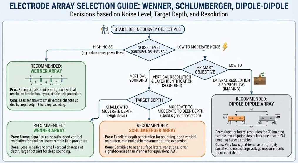
The Wenner array places four equally spaced electrodes in a straight line. It produces the strongest signal of all standard configurations for a given current. This high signal-to-noise ratio suits urban and industrial environments with strong interference. The Wenner array provides excellent vertical resolution for layered geology. Its main weakness is low lateral resolution and slow coverage speed. Engineers prefer Wenner for shallow engineering surveys and bedrock depth mapping.

2. Schlumberger Array

The Schlumberger array keeps potential electrodes fixed while expanding current electrode spacing. It achieves greater depth of investigation with fewer electrodes than Wenner. The apparent resistivity curve supports one-dimensional vertical sounding at a single point. This configuration is efficient for groundwater exploration and regional reconnaissance. It delivers better lateral resolution than Wenner at equivalent depth. The method’s main limitation is reduced resolution for complex 3D structures.

3. Dipole-Dipole Array

The Dipole-Dipole array separates current and potential pairs by a distance n times the dipole length. It delivers the highest lateral resolution of all standard configurations. This array excels at detecting steeply dipping contacts, faults and karst cavities. Its weakness is rapid signal decay, which reduces depth capability in conductive ground. The array is preferred for structural mapping and anomaly delineation.

4. Array Comparison and Selection Criteria

No single array performs best in every project scenario. The following matrix supports data-driven array selection.

Criterion	Best Array Choice	Reason
Noisy urban environment	Wenner	Highest signal-to-noise ratio
Deep groundwater sounding	Schlumberger	Maximum depth with few electrodes
Fault and cavity mapping	Dipole-Dipole	Best lateral resolution
Layered shallow geology	Wenner	Strong vertical resolution
Combined 2D/3D imaging	Hybrid (Wenner-Schlumberger)	Balanced resolution and signal

Hybrid arrays combine multiple configurations in a single acquisition sequence. Modern instruments switch array types automatically without moving electrodes. This flexibility lets field crews optimize data quality for local conditions.

Ⅳ. Resistivity Meters vs Other Geophysical Instruments

1. Cross-Method Comparison Matrix

Resistivity meters compete and complement with GPR, seismic and electromagnetic systems. Each technology measures different physical properties with distinct depth-resolution trade-offs.

Parameter	Resistivity Meter	GPR	Seismic	TEM
Physical Property	Resistivity	Dielectric constant	Elastic velocity	Conductivity
Typical Depth	5 – 1,500 m	0.1 – 30 m	5 – 500+ m	20 – 800 m
Lateral Resolution	0.5 – 10 m	0.02 – 0.3 m	1 – 5 m	5 – 20 m
Ground Contact	Yes (electrodes)	No	Yes (geophones)	No
Clay-Rich Soils	Works well	Poor penetration	Works well	Works well
Relative Cost	Low – Medium	Low	Medium – High	Medium – High

Resistivity meters offer the best balance of depth, resolution and cost for most engineering applications. GPR wins where centimeter-scale shallow resolution matters more than depth. Seismic methods dominate when mechanical properties of the ground are required. TEM penetrates deep conductive terrains where resistivity systems face logistics limits.

2. Synergy Strategies for Integrated Surveys

Combining resistivity with complementary methods reduces interpretation ambiguity. ERT and GPR joint surveys detect both structural and shallow high-resolution targets. Seismic plus resistivity integration is standard in mineral and geothermal exploration. Integrated surveys typically reduce total exploration risk more than drilling-only programs. The combined datasets calibrate each other and produce higher-confidence models.

Ⅴ. Industrial Applications

1. Mineral Exploration

Resistivity meters identify ore bodies through resistivity contrast with host rocks. Sulfide mineralization often produces low-resistivity anomalies in resistive host formations. High-power systems with IP capability extend effective exploration depth beyond 500 meters. The method also maps overburden thickness before drilling programs. Integration with magnetic and IP data improves targeting of economic mineralization.

2. Geotechnical and Urban Engineering

Resistivity surveys characterize ground conditions between boreholes with minimal disturbance. They detect karst cavities, fracture zones and weak layers before construction. Time-lapse surveys monitor groundwater changes and settlement during tunneling. Dam safety programs use repeat surveys to track seepage and internal erosion. The method supports road collapse risk assessment in urban corridors.

3. Hydrogeology and Environmental Monitoring

Resistivity mapping delineates aquifer geometry and groundwater quality zones. Fresh and saline groundwater produce strong resistivity contrasts in coastal areas. Time-lapse ERT tracks contaminant plume migration at industrial sites. The method monitors leachate movement at landfills without intrusive drilling. It is a standard tool for groundwater resource assessment and protection programs.

4. Archaeology and Specialized Applications

Resistivity surveys reveal buried structures through contrast with surrounding soil. They locate buried foundations, tombs and ancient settlement boundaries. The non-destructive nature makes resistivity ideal for heritage site investigation. Specialized applications include permafrost monitoring and soil salinity mapping.

Ⅵ. Buying Guide and Budget Framework

1. Specification Checklist for Buyers

Define survey objectives and target depth before comparing instrument models. Verify channel count against planned survey scale and productivity requirements. Check transmitter power against ground resistance in the project region. Confirm IP measurement capability if sulfide exploration is planned. Review software maturity for inversion and 3D modeling workflows.

2. Budget Tiers and Typical Configurations

Instrument costs vary widely with capability and channel count. The following table summarizes typical configuration tiers for planning purposes.

Budget Tier	Typical Configuration	Channel Count	Best Suited For
Entry Level	Portable resistivity meter	4 – 48	VES sounding, teaching, small projects
Mid Range	High-density ERT system	48 – 120	Engineering site surveys, karst mapping
High End	High-power IP-capable system	120 – 256+	Deep mineral, geothermal and 3D surveys

Budget estimates are indicative only and vary by brand and configuration. Always request reference projects and field demonstrations from suppliers. Include cables, electrodes, software and training in total cost calculations.

Ⅶ. Data Quality and Field Workflow

1. Standard Field Survey Workflow

A disciplined workflow ensures reliable resistivity data from planning to interpretation. First, design the survey based on target depth, resolution and site geology. Second, lay out electrodes with accurate spacing and good ground coupling. Third, measure contact resistance at each electrode before acquisition. Fourth, acquire data with defined current levels and stacking parameters. Finally, process, invert and interpret data with documented quality checks.

2. Quality Control and Data Validation

Quality control separates credible surveys from misleading interpretations. Contact resistance below 5kΩ is generally required for stable measurements. Repeat 5–10% of stations to quantify data repeatability and drift. Calibrate inverted models against borehole logs where available. Document environmental conditions and interference sources during acquisition.

Related Article

Title	Core Content	URL
What Are Resistivity Meters? Comprehensive Guide	Resistivity meter definition, working principle, electrode arrays and applications	https://geotechcn.net/service/what-are-resistivity-meters/
What is an Electrical Resistivity Meter?	Electrical resistivity meter principles, applications and ERT relationship	https://geotechcn.net/service/electrical-resistivity-meter/
Resistivity Meters: Precision Tools for Electrical and Geological Applications	Resistivity measurement principles and professional applications	https://geotechcn.net/service/resistivity-meters-ert/
What is a Resistivity Meter? 2D/3D Electrical Resistivity Imaging	Resistivity meters, ERT/ERI and high-density electrical methods	https://geotechcn.net/service/what-is-a-resistivity-meter-exploring-2d-3d-electrical-resistivity-imaging-techniques/
Resistivity Surveying Techniques	VES, high-density resistivity, 2D/3D ERI and ERT comparison	https://geotechcn.net/service/resistivity-surveying-techniques/
What Is an ERT Instrument?	ERT instruments, high-density resistivity, DC sounding and IP	https://geotechcn.net/service/ert-instruments/
ERT Equipment: Technology, Applications & Selection Guide	ERT system architecture, acquisition and equipment selection	https://geotechcn.net/service/ert-equipment/
Electrical Resistivity Tomography: A Complete Technical Guide	ERT physics, electrode configurations, acquisition and inversion	https://geotechcn.net/service/electrical-resistivity-tomography-a-complete-technical-guide/
What Is Electrical Resistivity Tomography (ERT)?	ERT fundamentals, 2D/3D imaging and applications	https://geotechcn.net/service/what-is-electrical-resistivity-tomography-ert/
What is Induced Polarization (IP) Method?	IP physics, acquisition, interpretation and applications	https://geotechcn.net/service/what-is-induced-polarization-ip-method-a-comprehensive-technical-guide/
A Comprehensive Guide to Electrical Resistivity Tomography	ERT methods, applications and data interpretation	https://geotechcn.net/service/geophysical-methods-ert-guide/
Geophysical Exploration Classification	Classification and relationship of electrical and other geophysical methods	https://geotechcn.net/service/geophysical-exploration-classification/

Reference Sources

Title	Core Content	URL
Electrical Resistivity — U.S. EPA	Four-electrode resistivity measurement, apparent resistivity, geometric factors, electrode arrays, DOI and inversion	http://www.epa.gov/environmental-geophysics/electrical-resistivity
Standard Guide for Using the Direct Current Resistivity Method for Geophysical Site Investigation — ASTM D6431-25	Professional guidance for DC resistivity site investigation, interpretation limitations and safety considerations	http://store.astm.org/d6431-25.html
Electrical Resistivity Tomography Data — USGS	Real-world ERT acquisition, electrode spacing, RTK positioning, processing and inversion	http://www.usgs.gov/data/electrical-resistivity-tomography-ert-data-collected-march-14-18-2022-and-november-17-21-2025
Electrical Resistivity Tomography — EarthScope Consortium	Practical ERT setup, resistivity meter, electrodes, current injection and apparent resistivity	http://www.earthscope.org/what-is/near-surface-geophysics/electrical-resistivity-tomography/
Electrical Resistivity — IEEE Technology Navigator	Four-electrode measurement principles, Wenner array, Schlumberger and dipole-dipole configurations	http://technav.ieee.org/topic/earth-resistivity/

---

FAQ