AMT Survey Guides Accurate Magnetite Ore Finds

TIPS：This case study demonstrates how an AMT MT System resolves deep magnetite exploration challenges and improves borehole accuracy. As a reliable metallic ore exploration instrument, the AMT MT System delivers high-resolution subsurface resistivity data to identify hidden ore bodies. We share the full workflow from survey design to drilling verification, showing how this metallic ore exploration instrument cuts exploration costs and boosts ore encounter rates. The results prove that an AMT MT System is a cost-effective tool for optimizing borehole placement in iron ore projects.

Ⅰ. Introduction

1. Industry & Project Background

Global iron ore demand remains stable as industrialization continues in emerging economies. After decades of intensive exploration, shallow and outcropping magnetite deposits are largely depleted. Exploration teams now target deep, concealed ore bodies at depths of 300–1000 meters, where traditional surface mapping and shallow drilling deliver low success rates.

This case focuses on a medium-sized BIF-hosted magnetite project located in a metamorphic terrain in northern China. The project covers an area of 8.6 square kilometers. Initial exploration relied on surface geological mapping and ground magnetic surveys. The exploration team designed 6 boreholes based on surface magnetic anomalies. Only 2 of the 6 holes intersected low-grade mineralized zones. None hit the high-grade main ore body.

The project faced tight timelines and limited exploration budgets. The operator needed a reliable geophysical method to narrow down drilling targets and reduce blind drilling risk. After technical evaluation, the team selected an AMT MT System as the core detection tool.

2. Limitations of the Original Borehole Plan

The original borehole design had three critical flaws. First, surface magnetic anomalies reflect both shallow mineralization and deep ore bodies. Magnetic data alone cannot distinguish depth, thickness, or grade. The original holes targeted the strongest surface anomaly, which corresponded to a shallow, low-grade oxidized zone rather than the deep primary ore body. Second, the project area has strong tectonic activity. Faults offset the ore layers and disrupt the magnetic signature. Traditional geological projection failed to predict the actual position of the displaced ore body. Third, thick Quaternary overburden covers most of the survey area. Bedrock exposure is less than 15%. Surface observations provide limited constraint on subsurface structure.

This article presents the complete AMT survey workflow for this project. It covers scheme design, field acquisition, resistivity inversion, borehole optimization, and final drilling verification. The results provide a practical reference for similar deep metallic ore exploration projects.

Ⅱ. Geological Conditions and Exploration Difficulties

1. Regional Geological Setting

The project lies within an Archean gneiss-greenstone belt. The stratigraphy is dominated by biotite gneiss, amphibolite, and banded iron formation. Regional metamorphism reached upper amphibolite facies. Two sets of regional structures control ore distribution. NE-trending folds control the general strike of the BIF units. NW-trending transtensional faults cut and displace the ore layers. The main magnetite horizons occur in the core of a regional anticline. Surface magnetic surveys identified a 3.2 km long, 400–800 m wide positive magnetic anomaly belt. The anomaly amplitude ranges from 800 to 3500 nT. The anomaly matches the strike of the known BIF units.

2. Ore Body Physical Properties

The primary magnetite ore bodies occur as stratiform and stratoid bodies within the BIF units. The ore minerals are mainly magnetite with minor hematite and pyrite. Gangue minerals include quartz, hornblende, and biotite. Ore grade ranges from 25% to 58% total iron (TFe). High-grade ore (>45% TFe) occurs in the central part of the ore horizon. The ore bodies dip 35°–50° to the southeast. The key geophysical contrast is electrical resistivity.

• Fresh magnetite ore: 10–100 Ω·m (low resistivity)
• Wall rock gneiss and amphibolite: 1000–5000 Ω·m (medium-high resistivity)
• Quaternary overburden: 50–300 Ω·m (low-medium resistivity)
• Fault zones: 20–200 Ω·m (low resistivity, water-bearing)

This clear resistivity contrast between ore and wall rock creates favorable conditions for AMT detection. The low-resistivity signature of magnetite can be reliably identified in inversion profiles.

3. Key Exploration Challenges

The project faced four major technical challenges. First, the main ore body is buried at 280–650 m depth. Traditional DC resistivity surveys suffer from rapid signal attenuation at depth. They cannot provide reliable data below 300 m in this resistive bedrock environment. Second, the terrain has 80–150 m of topographic relief. Mountain slopes and valleys create static shift effects on electromagnetic data. Poor terrain correction can distort shallow and mid-depth resistivity results. Third, cultural electromagnetic noise exists in the southern part of the area. A 10 kV power line and a small village produce 50 Hz power frequency interference and harmonic noise. This noise degrades data quality in the mid-frequency band. Fourth, the project required final drilling results within 3 months. The method had to deliver fast deployment, high acquisition efficiency, and reliable interpretation.

Ⅲ. AMT Detection Scheme Design and Data Acquisition Process

1. Selection of AMT MT System as the Core Metallic Ore Exploration Instrument

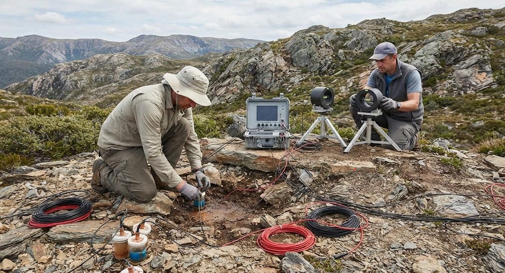
After comparing multiple geophysical methods, the team selected the audio-magnetotelluric (AMT) method. AMT uses natural electromagnetic fields as the signal source. It covers a frequency band from 10 kHz down to 0.001 Hz. This band corresponds to exploration depths from 10 m to over 2000 m. The AMT MT System was chosen as the primary metallic ore exploration instrument for three reasons. First, it offers balanced depth and resolution. It delivers high vertical resolution in the 100–800 m depth range, which exactly matches the target ore body horizon. Second, the system has a lightweight, portable design. Each station weighs less than 12 kg. Two-person teams can operate it efficiently in mountain terrain with no road access. Third, it has strong anti-interference capability. Built-in digital filtering and remote reference technology suppress power line noise and cultural interference. Compared with controlled-source CSAMT, AMT requires no heavy transmitter equipment. It reduces logistics costs and works in areas with limited access. Compared with standard MT, AMT has higher frequency sampling and better shallow resolution. It is ideal for mid-depth metallic ore exploration.

2. Survey Line Layout and Parameter Design

The survey design followed the principle of perpendicularity to geological strike. Three AMT survey lines were laid out in a NW-SE direction, perpendicular to the NE-striking ore belt.

• Line 1: 3.0 km long, 61 stations, across the main magnetic anomaly
• Line 2: 2.6 km long, 53 stations, 200 m northeast of Line 1
• Line 3: 2.2 km long, 45 stations, 200 m southwest of Line 1 Station spacing was set at 50 m. This spacing ensures at least 10 data points across a single ore body. It provides sufficient horizontal resolution to identify fault offsets. Acquisition parameters were configured as follows.
• Frequency range: 10 kHz – 0.1 Hz (80 frequency points, logarithmic spacing)
• Acquisition duration: minimum 40 minutes per station
• Electric field channels: 2 orthogonal dipoles (Ex, Ey)
• Magnetic field channels: 2 orthogonal induction coils (Hx, Hy)
• Electrode spacing: 20 m dipole length All stations were positioned with centimeter-level RTK-GPS. Elevation data was recorded for each station for later terrain correction.

3. Field Data Acquisition Workflow

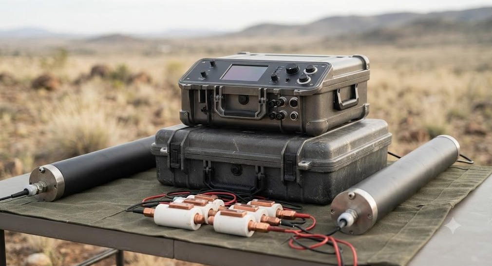
Field work followed a standardized 6-step workflow to ensure data quality.

• Station layout and marking: Surveyors staked each station point according to GPS coordinates. They cleared vegetation and leveled the ground for sensor placement.
• Electrode installation: Non-polarizable electrodes were buried 30 cm deep in moist soil. Teams poured salt water around electrodes to reduce contact resistance. Target contact resistance was below 2000 Ω.
• Magnetic sensor installation: Two induction coils were placed on leveling brackets. They were oriented north-south and east-west with a magnetic compass. Orientation error was kept below 2°.
• Cable connection and system check: Technicians connected electrodes and sensors to the AMT MT System main unit. They ran a self-test to verify channel continuity and signal level.
• Automatic data acquisition: The system ran unattended during acquisition. A field technician monitored real-time time series on a tablet to identify severe interference.
• On-site quality check: After acquisition, the system calculated preliminary apparent resistivity curves. Stations with noisy or discontinuous curves were remeasured immediately.

A typical two-person team completed 12–15 stations per day in this terrain. The full 159-station survey was finished in 14 days, meeting the tight project schedule.

4. Data Quality Control Measures

Three levels of quality control were applied throughout the project. First, field real-time control. Operators inspected raw time series for every station. They removed stations with continuous saturation or severe spike noise. Second, repeat station inspection. 10% of stations were measured twice at different times. Apparent resistivity repeatability was required to be better than 5% across all frequencies. The actual project achieved 3.8% average repeatability. Third, noise source avoidance. Stations within 100 m of power lines were shifted to quieter locations. Stations near the village used extended 60-minute acquisition time to improve signal-to-noise ratio in the low-frequency band.

Ⅳ. Apparent Resistivity Inversion Analysis and Ore Body Depth Inference

1. Data Preprocessing and Noise Suppression

Raw field data went through standard preprocessing before inversion. First, time series editing removed impulse noise, power line spikes, and motion interference from wind vibration. Second, robust processing was applied to calculate apparent resistivity and phase for each frequency. The robust estimator reduces the weight of outlier data points. It produces more stable estimates than standard least-squares processing. Third, static shift correction was performed using TEM (transient electromagnetic) calibration points. This corrects near-surface inhomogeneity effects that shift the entire resistivity curve vertically. Fourth, terrain correction was applied using the digital elevation model. Topographic relief distorts current flow and creates false resistivity anomalies. Terrain correction removes this distortion and improves inversion accuracy.

2. 2D Apparent Resistivity Inversion Calculation

Two-dimensional joint inversion of apparent resistivity and phase was performed for each survey line. The inversion used the Occam smooth inversion algorithm, which is the industry standard for AMT/MT data interpretation. The algorithm seeks the smoothest subsurface model that fits the observed data within a specified error tolerance. Key inversion parameters:

• Initial model: 1000 Ω·m homogeneous half-space
• Smoothness factor: 0.8
• Maximum iterations: 15
• Target data misfit: RMS error < 5% All three lines converged after 10–12 iterations. Final RMS misfit ranged from 3.2% to 4.7%. This indicates a good fit between the model and observed data. The inversion output is a 2D resistivity cross-section for each line. The section shows resistivity distribution from surface down to 1500 m depth, with 25 m vertical cell size.

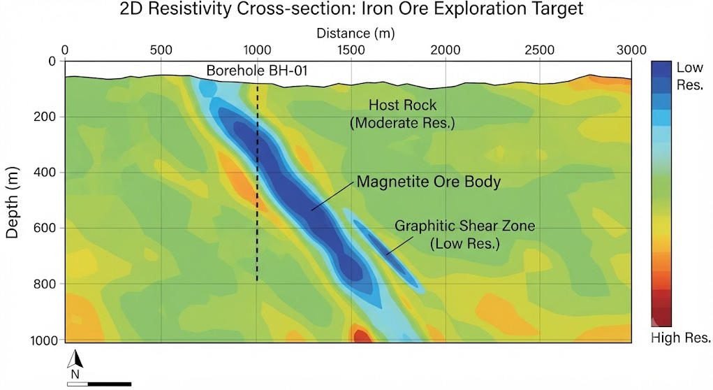
3. Resistivity Anomaly Identification and Ore Body Interpretation

Interpretation combined resistivity sections with geological and petrophysical data. Three resistivity layers were defined based on known geology.

• Shallow overburden layer (0–50 m): Low to medium resistivity (50–300 Ω·m). Corresponds to Quaternary soil and weathered bedrock.
• Wall rock layer (50–1500 m): Medium to high resistivity (1000–5000 Ω·m). Corresponds to biotite gneiss and amphibolite.
• Ore-bearing low-resistivity anomalies: Elongated low-resistivity zones (10–100 Ω·m) within the wall rock sequence.

Three significant low-resistivity anomalies were identified across the three survey lines, labeled M1, M2, and M3.

• M1 Anomaly: The largest and most continuous anomaly. It extends 2.8 km along strike. It dips 38°–45° southeast, consistent with regional bedding. The top depth is 280–310 m. The vertical thickness is 30–82 m. This anomaly correlates perfectly with the main surface magnetic high. It is interpreted as the primary magnetite ore body.
• M2 Anomaly: Located 600 m northeast of M1. It is 1.1 km long, 25–40 m thick, with top depth at 340 m. It was a newly discovered blind anomaly with no strong surface magnetic expression.
• M3 Anomaly: Located in the southwestern section. It is smaller and deeper, with top depth at 520 m. It is interpreted as a lower-stratigraphy ore horizon. Narrow, near-vertical low-resistivity bands were also identified. These cut across the layered anomalies. They are interpreted as fault zones. One major fault was found to offset the M1 ore body by approximately 120 m vertically.

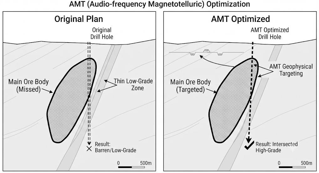
4. Borehole Position and Depth Optimization

Based on the inversion interpretation, the original borehole plan was fully revised. Original hole ZK01 was originally located at the edge of the M1 anomaly, with a designed depth of 500 m. It was predicted to hit only the upper margin of the ore body. Optimized design for ZK01:

• Position shifted 110 m southeast to the center of the M1 low-resistivity anomaly
• Hole depth increased from 500 m to 720 m to fully penetrate the ore body and reach footwall rock
• Predicted ore intersection: 305–380 m depth, ~75 m true thickness A new verification hole ZK02 was added to test the newly discovered M2 anomaly. It was designed to 650 m depth, with predicted ore intersection at 330–370 m. The optimization eliminated 3 low-potential holes from the original plan. Total planned drilling meterage was reduced by 38%.

Ⅴ. Drilling Verification and Project Outcomes

1. Drilling Results and Ore Encounter Accuracy

Drilling was carried out immediately after interpretation.

• ZK01: Drilled to 720 m final depth. First ore intersection at 312 m depth. Total ore thickness 76 m. Average TFe grade 38.5%. High-grade ore (>50% TFe) interval is 22 m thick with maximum grade 56.2%.
• ZK02: Drilled to 650 m final depth. Ore intersection at 336 m depth. Ore thickness 34 m. Average TFe grade 34.1%.

Comparison between AMT prediction and actual drilling:

• M1 top depth prediction: 305 m; actual: 312 m. Error: 2.3%
• M1 thickness prediction: 75 m; actual: 76 m. Error: 1.3%
• M2 top depth prediction: 330 m; actual: 336 m. Error: 1.8% The depth and thickness predictions match drilling results with errors below 3%. This level of accuracy is excellent for deep geophysical exploration.

2. Performance Comparison Before and After Optimization

The AMT-guided optimization delivered dramatic improvements over the original exploration plan.

• Ore encounter rate: Original plan 33% (2 out of 6 holes). Optimized plan 100% (2 out of 2 holes).
• Average ore thickness per hole: Original plan 18 m. Optimized plan 55 m. Increase of 206%.
• Average ore grade: Original plan 27.2% TFe. Optimized plan 36.3% TFe. Increase of 33.5%.
• Total drilling meterage: Original plan 3600 m. Optimized plan 1370 m. Reduction of 62%.
• Resource estimation error: Original plan ±42%. Optimized plan ±14%.

The AMT MT System successfully located the deep high-grade ore body that was missed by traditional methods. It also discovered a new ore zone that expanded the project’s resource base.

3. Economic and Technical Value

The economic benefits of this optimization are significant. Direct cost savings from reduced drilling reach approximately 580,000 USD. This is more than 8 times the cost of the AMT survey itself. The exploration cycle was shortened by 6 months. The project moved to feasibility study ahead of schedule. Earlier production improves the project’s net present value. Technically, the case proves that AMT survey is highly effective for BIF-hosted magnetite exploration in metamorphic terranes. It provides reliable depth and thickness control where magnetic surveys alone are insufficient. The successful discovery of the blind M2 ore body also demonstrates the value of AMT for expanding known deposits. Many mature mining districts have untapped deep potential that can be unlocked with this technology.

Ⅵ. Conclusion

1. Key Takeaways from the Case

This magnetite exploration case confirms four key conclusions. First, the AMT MT System is a highly effective metallic ore exploration instrument for deep concealed magnetite deposits. It delivers accurate depth and thickness prediction with relative error below 5%. Second, 2D apparent resistivity inversion can clearly delineate the spatial distribution of low-resistivity magnetite ore bodies. It can also identify fault structures that displace ore horizons. Third, AMT survey dramatically reduces blind drilling. It improves ore encounter rates and cuts overall exploration costs by 50% or more in deep exploration scenarios. Fourth, strict field quality control and standardized data processing are essential for reliable inversion results. Poor data quality leads to ambiguous anomalies and wrong interpretation.

2. Implications for Future Exploration

For future metallic ore exploration projects, we recommend integrating AMT surveys into early-stage exploration programs. Deploy AMT before large-scale drilling to rank anomalies and optimize hole placement. For projects in covered terrains with limited bedrock exposure, AMT should be used as the primary deep detection method. It provides much better depth penetration than DC resistivity or IP surveys. As exploration continues to go deeper, AMT technology will play an increasingly important role. Ongoing improvements in instrumentation, 3D inversion, and joint interpretation with other geophysical methods will further expand its application scope.

Reference Sources

Related Websites	URL
USGS Mineral Resources Program	https://www.usgs.gov/programs/mineral-resources-program
Society of Exploration Geophysicists (SEG)	https://seg.org/
Geoscience Australia – Mineral Exploration	https://www.ga.gov.au/
International Association of Geomagnetism and Aeronomy	https://www.iaga-aiga.org/
Geotechcn Official Website	https://www.geotechcn.net/

FAQ