What is ERT？丨Guide to ERT Principles, Arrays, and Subsurface Imaging

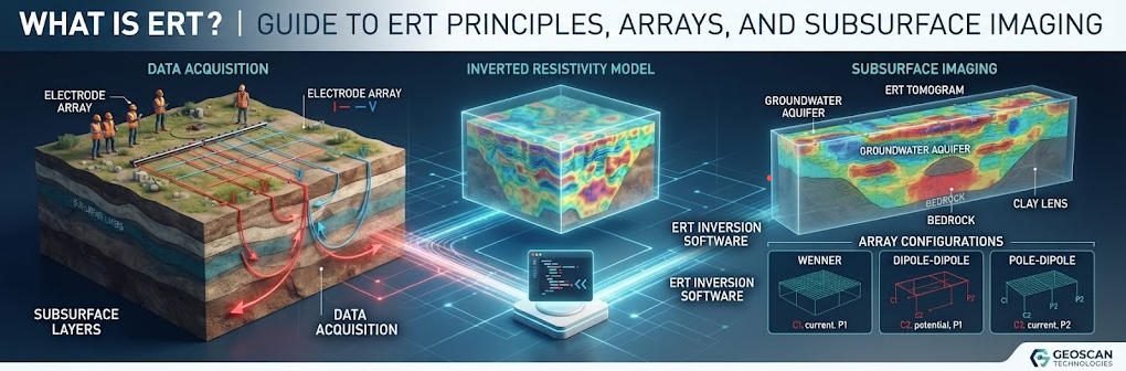
TIPS：Electrical resistivity tomography (ERT) images subsurface structures by injecting direct current through electrode arrays and measuring voltage differences. This guide explains ERT principles, geometric factors, and array configurations including Wenner, Schlumberger, and dipole-dipole. Engineers learn survey design, 2D versus 3D acquisition, inversion workflows, and quality control for groundwater, environmental, and geotechnical applications.

I. Fundamentals of Electrical Resistivity Tomography

1. Definition and Scope

Electrical resistivity tomography (ERT) is a geophysical method that images subsurface resistivity distribution by injecting direct current through surface electrodes and measuring resulting voltage differences. It produces two-dimensional cross-sections or three-dimensional volumetric models of the ground. Unlike vertical electrical sounding, which yields only one-dimensional depth profiles at discrete points, ERT captures lateral variations continuously along a survey line or across a grid.

The method is widely applied in groundwater exploration, environmental site characterization, mineral prospecting, and geotechnical engineering. Depending on electrode spacing and array configuration, investigation depths range from approximately one meter to several hundred meters. Resolution decreases with depth, making ERT most effective for targets within the upper 100 meters of the subsurface.

2. Physical Principles

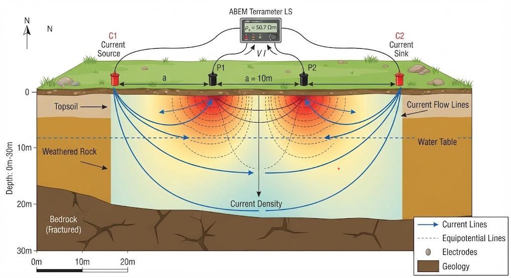
ERT operates on Ohm’s Law, which relates voltage, current, and resistance in an electrical circuit. Field crews inject a known direct current into the ground through two current electrodes. Two separate potential electrodes measure the voltage drop at the surface. The instrument calculates resistance from these values.

Resistance alone does not describe the material. It depends on electrode geometry and current path. To obtain a material property, engineers multiply measured resistance by a geometric factor. This yields apparent resistivity, which represents the bulk electrical response of the ground volume sampled by that specific electrode configuration.

Apparent resistivity differs from true resistivity. True resistivity is the intrinsic property of a specific geological layer. Apparent resistivity is what the instrument measures, assuming a homogeneous half-space. Inversion algorithms convert apparent resistivity data into true resistivity models by accounting for layered and heterogeneous subsurface conditions.

3. Factors Controlling Resistivity

Subsurface resistivity depends on multiple physical and chemical properties. Pore water content exerts the strongest influence. Saturated zones exhibit low resistivity because water conducts electricity. Dry rock or frozen ground shows high resistivity. Clay minerals further reduce resistivity through surface conduction along particle boundaries.

Fluid chemistry also matters. Fresh groundwater typically ranges from 10 to 100 ohm-meters. Saline water or contaminated plumes may drop below 1 ohm-meter. Metallic sulfides and graphite create extremely low resistivity zones. Depending on mineralogy and saturation, common earth materials span several orders of magnitude.

Material Type	Typical Resistivity Range (Ω·m)	Key Influencing Factor
Clay and saturated silt	1–20	High surface conduction; pore water
Sand and gravel (freshwater)	50–500	Porosity; pore fluid resistivity
Sand and gravel (saline)	2–20	Salinity dominates
Weathered granite	50–500	Fracture density; moisture content
Fresh granite/gneiss	1,000–10,000	Low porosity; minimal water
Limestone (compact)	500–5,000	Porosity; karst development
Saltwater	0.1–1	Ionic concentration
Ice/permafrost	1,000–100,000	Absence of liquid water

II. Electrode Arrays and Survey Design

1. The Geometric Factor

The geometric factor normalizes measured resistance for electrode geometry. It depends on the relative positions of current and potential electrodes. For a four-electrode array, the factor converts resistance into apparent resistivity using the formula: apparent resistivity equals resistance multiplied by the geometric factor.

Different array types produce different geometric factors. Wenner arrays use equal spacing between all four electrodes. Schlumberger arrays maintain a fixed potential electrode pair while moving current electrodes outward. Dipole-dipole arrays separate current and potential pairs by a fixed distance. Each configuration samples the subsurface differently, creating distinct sensitivity patterns.

2. Wenner Array

The Wenner array is the simplest configuration. All four electrodes are equally spaced at distance “a”. Current electrodes occupy the outer positions, and potential electrodes sit between them. The geometric factor for Wenner is straightforward: two times pi times electrode spacing.

Wenner arrays offer strong signal amplitude and good vertical resolution. They perform well in layered geology where horizontal boundaries dominate. However, the fixed spacing requires more electrodes to achieve deep penetration. Depending on target geometry, Wenner may miss steeply dipping structures because current flows predominantly horizontally.

3. Schlumberger Array

Schlumberger arrays place potential electrodes close together near the center, with current electrodes at much wider separations. The geometric factor changes as current electrodes move outward. This design maintains a relatively constant sensitivity volume while increasing depth penetration.

The Schlumberger configuration requires fewer electrodes than Wenner for deep surveys. It offers excellent vertical resolution and works well for depth sounding along a profile. Signal strength decreases at large separations, so high-power transmitters become necessary for deep targets. Depending on ground resistivity, current injection may require voltages up to several hundred volts.

4. Dipole-Dipole Array

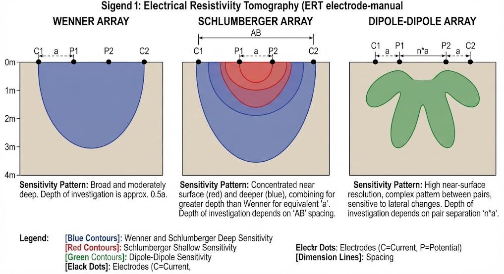
Dipole-dipole arrays separate current and potential electrode pairs by a fixed multiple of the dipole length. This configuration is highly sensitive to lateral resistivity contrasts. It excels at mapping vertical structures such as faults, dikes, and fracture zones.

The dipole-dipole array produces weaker signal amplitudes than Wenner or Schlumberger. It is more susceptible to noise from cultural sources and telluric currents. However, its superior lateral resolution makes it the preferred choice for complex geological environments where steeply dipping targets are expected.

Array Type	Signal Strength	Vertical Resolution	Lateral Resolution	Noise Susceptibility	Best Application
Wenner	Strong	Good	Moderate	Low	Layered geology; shallow engineering
Schlumberger	Moderate to strong	Excellent	Moderate	Low to moderate	Deep groundwater; bedrock mapping
Dipole-dipole	Weak	Moderate	Excellent	High	Faults; karst; mineralized veins
Pole-dipole	Moderate	Good	Good	Moderate	Asymmetric structures; 3D coverage
Gradient	Strong	Moderate	Good	Low	Large-area reconnaissance

5. Hybrid and Optimized Configurations

Modern multi-electrode systems collect data using multiple array types in a single deployment. Hybrid configurations combine Wenner and dipole-dipole measurements to leverage the strengths of each. Optimized arrays use computer algorithms to select electrode combinations that maximize sensitivity to specific target geometries.

The choice of array depends on target depth, expected geometry, noise environment, and time constraints. For routine environmental surveys, Wenner-Schlumberger hybrids provide a good balance. For mineral exploration, dipole-dipole or pole-dipole configurations often prove more diagnostic.

III. Two-Dimensional vs. Three-Dimensional ERT

1. Two-Dimensional Surveys

Two-dimensional ERT deploys electrodes along a single linear profile. The inversion algorithm assumes that subsurface geology does not change significantly perpendicular to the profile. This assumption holds reasonably well for linear features such as roads, pipelines, dams, and river crossings.

Two-dimensional surveys are faster and require less equipment than three-dimensional surveys. A typical 2D profile with 48 electrodes and 5-meter spacing covers 235 meters of surface length and images to approximately 40 to 50 meters depth. Data acquisition typically requires two to four hours depending on instrument channels and stacking parameters.

The main limitation is the out-of-plane assumption. If strong three-dimensional structures exist, 2D inversion produces artifacts and distorted resistivity values. Geophysicists must assess geological complexity before selecting a 2D approach.

2. Three-Dimensional Surveys

Three-dimensional ERT uses multiple parallel profiles or a surface grid of electrodes. The inversion algorithm solves for resistivity variations in all three spatial directions. This approach eliminates out-of-plane artifacts and provides true volumetric models.

Three-dimensional surveys require significantly more field time and electrodes. A modest 3D grid covering 100 by 100 meters with 5-meter spacing uses 400 electrodes. Data volumes are large, and inversion computation may require hours to days. Depending on project budget and timeline, 3D surveys cost five to ten times more than equivalent 2D coverage.

The benefits are substantial for complex sites. Karst terrain, ore bodies, landfill plumes, and building foundations often require 3D imaging for reliable interpretation. When drilling costs are high, the additional geophysical investment typically pays for itself through improved target definition.

Survey Dimension	Electrode Count	Field Time	Inversion Time	Best Use Case	Relative Cost
2D	24–96	2–6 hours	Minutes to hours	Linear structures; reconnaissance	Baseline
3D grid	200–1,000+	1–5 days	Hours to days	Complex geology; volumetric targets	5–10x
Cross-borehole 2D	16–48 per hole	4–8 hours	Hours	Deep fracture zones; tunnel walls	3–5x
Cross-borehole 3D	32–96 total	1–2 days	Days	Detailed deep characterization	8–15x

IV. Data Acquisition and Quality Control

1. Instrumentation

Modern ERT instruments use multi-channel acquisition systems. A single instrument may support 64 to 256 channels, enabling simultaneous measurement across many electrode combinations. This parallel architecture reduces field time dramatically compared to older single-channel systems.

Key instrument specifications include input impedance, measurement resolution, maximum output voltage, and current accuracy. Input impedance should exceed 100 megaohms to avoid loading effects on high-resistivity ground. Resolution of 0.1 millivolts or better ensures adequate signal detection in noisy environments.

2. Electrode Installation

Electrode contact resistance critically affects data quality. Steel stakes driven 10 to 30 centimeters into soil typically achieve contact resistances below 10 kiloohms. Dry sand, gravel, or frozen ground may require saltwater, bentonite mud, or deeper emplacement to achieve acceptable contact.

Multi-conductor cables connect electrodes to the switching unit. Cable capacitance and leakage can introduce errors, particularly in wet conditions. Regular cable inspection and connector cleaning reduce these problems. Depending on terrain, crews may need to clear vegetation or level electrode positions.

3. Noise Sources and Mitigation

ERT surveys are vulnerable to several noise sources. Power lines induce alternating current interference at 50 or 60 hertz. Metal fences, pipelines, and railways create galvanic and inductive disturbances. Telluric currents from ionospheric variations add low-frequency noise.

Mitigation strategies include increasing stacking repetitions, using notch filters, and selecting measurement times when cultural noise is minimal. Some instruments offer synchronous sampling that averages out periodic interference. In extreme cases, electrode arrays must be relocated away from noise sources.

Reciprocal measurements provide a powerful quality check. The instrument swaps current and potential electrodes and repeats the measurement. In a noise-free system, the reciprocal measurement equals the original. Large discrepancies indicate poor data quality at that electrode combination.

V. Inversion and Interpretation

1. Forward Modeling

Forward modeling predicts what ERT data would look like for a given subsurface resistivity model. It solves the governing partial differential equations for electrical potential distribution. Engineers use forward modeling to test hypotheses and design surveys before field deployment.

Finite-element and finite-difference methods are the standard numerical approaches. These divide the subsurface into discrete cells and solve for potential at each node. Mesh refinement near electrodes and target zones improves accuracy. Depending on model complexity, forward calculations require seconds to minutes.

2. Inversion Algorithms

Inversion converts measured apparent resistivity data into a true resistivity model. This is an ill-posed mathematical problem because multiple models can produce similar data. Regularization constraints stabilize the solution by penalizing unrealistic model roughness.

The most common approach is smoothness-constrained least-squares inversion. It minimizes an objective function that combines data misfit and model roughness. A trade-off parameter controls the balance between fitting the data and producing a smooth model. When geological boundaries are sharp, robust or L1-norm constraints may produce better results than standard L2 smoothness constraints.

Inversion Approach	Constraint Type	Best For	Risk
L2 smoothness	Standard least squares	Layered geology; gradual transitions	Blurs sharp boundaries
L1 robust	Absolute deviation minimization	Faults; karst; sharp contacts	May introduce artifacts
Structural	External boundary constraints	Sites with borehole or seismic data	Requires accurate prior information
Joint	Multi-method coupling	ERT plus GPR or seismic	Complex setup; cross-method calibration

3. Interpretation Guidelines

Interpreting ERT models requires geological knowledge and an understanding of method limitations. Resistivity values are non-unique. A low-resistivity zone could indicate clay, saline water, or metallic mineralization. Additional information from drilling, geology, or complementary geophysical methods reduces ambiguity.

Depth scales on ERT sections are approximate. The depth to a given boundary depends on the resistivity contrast and array type. Inversion artifacts commonly appear at depth and near profile ends. Geophysicists should evaluate model sensitivity and resolution maps before making definitive interpretations.

VI. Engineering and Environmental Applications

1. Groundwater and Hydrogeology

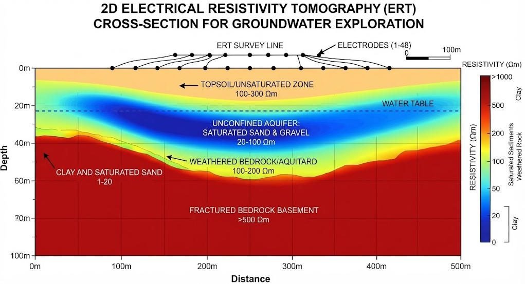
ERT is widely used to map aquifer geometry, water table position, and saline intrusion. Freshwater aquifers in sand and gravel typically show resistivities of 50 to 500 ohm-meters. Clay layers or saline zones appear as low-resistivity barriers or wedges. Time-lapse ERT monitors seasonal water table fluctuations and pumping impacts.

Fractured bedrock aquifers present a greater challenge. Water-bearing fractures may appear as narrow low-resistivity zones within high-resistivity rock. Depending on fracture orientation and aperture, ERT may or may not resolve individual features. Cross-borehole configurations improve detection in these cases.

2. Environmental Site Characterization

Environmental consultants use ERT to delineate contaminant plumes, landfill boundaries, and buried drums. Hydrocarbon spills often increase resistivity because oil displaces conductive groundwater. Saline or leachate plumes decrease resistivity. The method works best when baseline resistivity is known before contamination occurs.

ERT also monitors remediation progress. In-situ chemical oxidation, bioremediation, and thermal treatment alter subsurface chemistry and moisture. Repeated surveys track treatment front propagation and verify barrier integrity. Depending on plume complexity, 3D ERT may be necessary for accurate volumetric estimation.

3. Geotechnical Engineering

Civil engineers apply ERT to assess foundation conditions, detect voids, and map bedrock depth. Karst terrain poses significant construction risks because subsurface cavities may collapse under load. ERT identifies anomalous low-resistivity zones that often correspond to soil-filled sinkholes or fracture networks.

Dam and levee investigations use ERT to detect seepage pathways and internal erosion. Saturated zones within embankments show lower resistivity than intact fill material. However, ERT cannot quantify flow rates or hydraulic pressure. It must be combined with piezometric data for comprehensive dam safety assessment.

4. Mineral Exploration

Mineral exploration employs ERT to map alteration zones, sulfide bodies, and graphitic horizons. Sulfide minerals exhibit both low resistivity and high chargeability. Combined ERT and induced polarization surveys distinguish ore-related anomalies from barren conductive features.

Deep porphyry systems require large electrode spacings and high transmitter power. Three-dimensional ERT grids help define ore body geometry and guide drilling programs. Depending on overburden thickness and conductivity, ERT may be supplemented with electromagnetic or seismic methods.

VII. Limitations and Method Constraints

1. Resolution and Depth Trade-offs

ERT resolution is fundamentally limited by electrode spacing and physics. Near-surface features may resolve at sub-meter scale. At 50 meters depth, resolution degrades to 5 to 10 meters or worse. The depth of investigation rarely exceeds one-third to one-fifth of the total array length.

These constraints are inherent to the method. No instrument or inversion algorithm can overcome the physics of diffuse current flow. Survey designers must accept these limits and select electrode configurations appropriate for target size and depth.

2. Site Constraints

ERT requires galvanic contact with the ground. Paved surfaces, solid rock outcrops, and frozen terrain complicate electrode installation. In urban environments, buried utilities, metal fences, and electromagnetic interference degrade data quality.

Steep topography distorts current flow and requires topographic correction in inversion. Dense vegetation may obstruct cable deployment. Depending on site conditions, these constraints may preclude ERT or require modified field procedures such as capacitive coupling or borehole deployment.

3. Interpretation Ambiguity

Resistivity models are non-unique. Different geological scenarios can produce similar ERT responses. Clay, water, and sulfides all appear as low-resistivity zones. Without geological control, interpreters risk misidentifying materials.

Quantitative interpretation requires petrophysical relationships calibrated to local conditions. Archie’s law relates resistivity to porosity and water saturation in clean sands. Clay-rich formations require more complex models. Depending on project requirements, borehole logging or laboratory measurements may be necessary for reliable conversion.

VIII. Survey Planning and Best Practices

1. Defining Objectives and Constraints

Effective ERT surveys begin with clear objectives. Target depth, expected geometry, and required resolution determine array type and electrode spacing. Budget and schedule constraints influence the choice between 2D and 3D approaches.

Geological and hydrogeological background information guides survey design. Existing boreholes, geological maps, and prior geophysical data help identify likely resistivity contrasts and potential noise sources. Pre-survey forward modeling tests whether the proposed configuration can resolve the target.

2. Field Procedures

Standard field procedures include electrode installation, contact resistance checking, and test measurements. Contact resistance should remain below 10 kiloohms for all electrodes. Higher values indicate poor contact and may require remediation.

Data acquisition proceeds automatically once parameters are set. The operator monitors data quality in real time, watching for abnormal values or high reciprocal errors. Bad data points are flagged for removal or re-measurement. Depending on survey length, daily progress typically ranges from one to three 2D profiles.

3. Reporting and Integration

Final deliverables include resistivity cross-sections or volumes, interpretation maps, and technical documentation. Reports should state assumptions, limitations, and uncertainty levels. Integration with drilling data, geological maps, and other geophysical methods strengthens interpretation confidence.

Modern practice favors digital delivery of inverted models in formats compatible with GIS and 3D visualization software. This enables engineers and geologists to integrate ERT results into broader site models and decision-making workflows.

Reference Sources

Name	Title	URL
U.S. EPA	Electrical Resistivity: Environmental Geophysics Technical Overview	https://www.epa.g-resistivity
CLU-IN (EPA)	Electrical Resistivity Tomography Technology Overview	https://clu-in.or_Tomography/
USGS CMGDS	Coastal and Marine Geosciences: Electrical Resistivity Data Catalog	https://cmgds.mar=2&term=2087
Springer / Surveys in Geophysics	Review on Applications of Time-Lapse ERT Over the Last 30 Years	https://link.spri-022-09731-2
MDPI / Applied Sciences	TL-ERT for Landslide Monitoring: Recent Advances and Future Directions	https://www.mdpi.17/12/3/1425

FAQ