Geophysical Methods: ERT Guide

Geophysical Methods: A Comprehensive Guide to Electrical Resistivity Tomography (ERT)

Introduction to Electrical Resistivity Tomography (ERT)

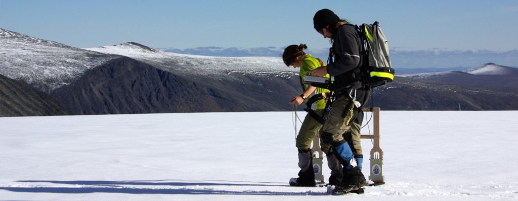
Electrical Resistivity Tomography (ERT) is a well-established and versatile geophysical technique that measures the spatial distribution and contrast of electrical resistivity in the subsurface. ERT measurements can be performed along a linear surface transect, in a grid or non-linear geometry, as a vertical sounding, in a borehole, or from watercraft. The data are used to produce a two-dimensional (2-D) electrical image (a “cross section” or “plane”) or three-dimensional (3-D) distribution of subsurface resistivity values, analogous to a medical CAT scan. Although there are many applications of ERT to a variety of industries, this technology area focuses on the surface line application (Figure 1).

Figure 1. Example of an Electrical Resistivity Survey Using a Fixed Linear Array.

Applications of ERT in Environmental Studies

ERT is commonly used in environmental applications to:

• Estimate depth, thickness, and resistivity of subsurface layers.
• Estimate depth to the water table.
• Identify boundaries of landfill and burial pit sites.
• Develop a broad, low-resolution cross section of the site.
• Reconcile boring logs from multiple drilling efforts over time and identification of data gaps requiring further investigation.
• Detect high-concentration contaminant plumes and variations in hydrogeological properties using temporal imaging.
• Detect injected amendment or microbial distribution in the subsurface.

ERT can reliably distinguish the upper four layers of discrete rock or soil types, with sufficient electrical resistivity contrast down to 100 meters (m) depending on the survey configuration. ERT is best applied in areas without common sources of signal interference or noise, including:

• Buried pipes, culverts, and cables.
• Metal fences and powerlines.
• Metal from nearby vehicles and buildings.
• Highly resistive ground (i.e., bedrock).

Typical Uses of Resistivity Surveys

Resistivity depends on mineral composition, structure of the subsurface material, porosity, and pore fluid composition, among other factors. For instance, loose sand can register between 1,000 to 100,000 Ohm-meters (Ω-m). Therefore, a resistivity survey works best to distinguish rock layers based on their relative resistivities. The greatest contrast in resistivity is most often seen between water-bearing and non-water-bearing geologic units. A resistivity survey is most effective at determining:

• Boundaries between subsurface layers of varying electrical properties.
• Extent of pore space saturation (depth of the water table).

Emerging uses of resistivity surveys include determining:

• Relative porosity and permeability of saturated subsurface materials based on field data and/or modeling.
• Locations of fault and fracture zones, caves, and changes in lithology.
• Changes in the subsurface characteristics over time using time-lapse ERT. Time-lapse ERT can also help monitor changes in aquifer quality.
• Concentration of dissolved electrolytes and colloids in pore fluid, which would require additional information on the geology to understand subtle differences in resistivity caused by the dissolved load in groundwater. Cross-hole ERT also has been used to increase sensitivity and resolution of these measurements with depth.

A resistivity survey can also rapidly and quantitatively reconcile different sets of qualitative boring log data. As such, a resistivity survey should always be correlated with borehole data to connect specific resistivity signatures with a particular rock or soil layer at the site.

Theory of Operation: How ERT Works

ERT works by transmitting a direct electrical current into the ground using a pair of current electrodes (see C1 and C2 in Figure 2) and then measuring the voltage at one or more additional pairs of potential electrodes along the straight survey line (see P1 and P2 in Figure 2). With the voltage (V) and current (I) known, the equivalent resistance (R) of the earth materials surveyed can then be calculated using Ohm’s Law:

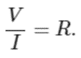
The equivalent resistance from this calculation assumes that the subsurface materials are uniform and homogeneous. In reality, the resistivity measured by the four-electrode configuration is determined by the various lithologies and subsurface structures which may be inhomogeneous. The applied current can take several paths through the subsurface. The inversion algorithm compares voltage readings for different electrode spacings to assign an “apparent resistivity” value to a particular depth. The geometry of the electrode spacing is an important factor in the design, analysis, and interpretation of an ERT survey. Resistance meters typically measure a resistance value, R as described in the above equation. Apparent resistivity is then calculated by multiplying this resistance by a geometric factor:

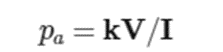
where pa is the apparent resistivity and k is the geometric factor based on the spacing of the participating electrodes.

Many electrode array configurations (the spacing of electrodes and their relative positions) may be used, but the most common arrays are the Wenner, Schlumberger, and dipole-dipole. The depth of measurement is controlled by the electrode spacing of the array (Table 1). As the spacing is increased, greater depths of measurement are reached. A survey length with maximum spacing of three to four times to depth of interest is recommended to adequately characterize layers at depth. In general, when electrodes are closer together, more of the current travels through shallower layers, and when electrodes are further apart, more of the current travels through deeper layers.

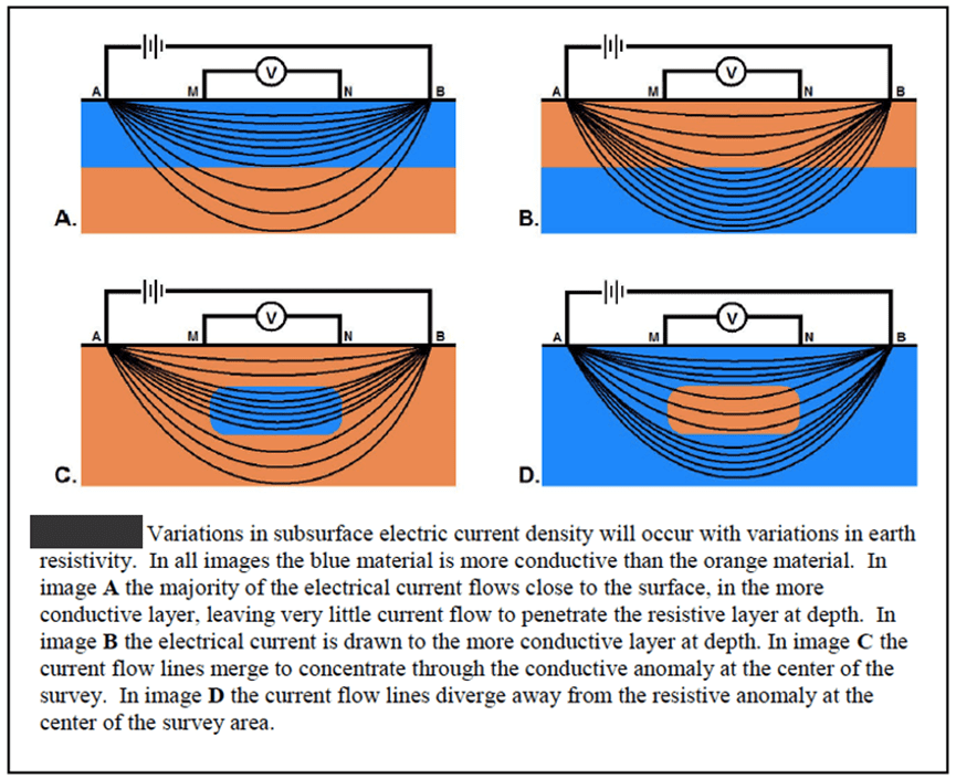
The path the applied electrical current takes in the subsurface will deviate from the theoretical movement of the applied electrical current, as shown in Figure 2. One complicating factor is that electrical current prefers to take the path of least resistance (Figure 3). As the number of discrete layers increases and horizontal heterogeneities emerge (Figure 3C and 3D), the current’s path becomes more convoluted, and the algorithm can return numerous solutions if not bound by sufficient borehole log data or other geophysical data.

System Components and Setup

A typical ERT system includes:

• 18-inch metal stake electrodes.
• 20- to 100-meter cables and clamp connectors.
• A resistivity meter powered by a portable battery.
• Bentonite clay and water or saltwater to improve ground contact in arid regions.

The setup process involves staking electrodes into the ground, connecting them to the cables, and programming the resistivity meter with the desired electrode array configuration. Surveys can be conducted in sounding mode (to gather data with depth) or profile mode (to collect lateral variations in resistivity).

Modes of Operation

This section focuses on the surface application of ERT, but electrical resistivity data also can be collected beneath water bodies using watercraft (Figure 4) and from the subsurface via boreholes. Detailed data at depth in the subsurface can be collected from a single borehole  cross-hole, or as a borehole-surface deployment where open spaces for surface deployment are limited.

A typical resistivity 2-D imaging survey involves two cables extending from the resistivity meter in opposite directions. The field crew stakes electrodes 12 inches into the ground and connects them to the cables. Typically, the electrodes are spaced 5 or 10 meters apart. A particular “array,” or electrode configuration, must be programmed into the resistivity meter. The Schlumberger and Wenner arrays are frequently used for imaging since they are sensitive to vertical variations in subsurface resistivity and less affected by noise, though less sensitive to horizontal variations.

Surveys are conducted in a sounding mode, profile mode, or both. In sounding mode, the distance between electrodes is increased while the center of the array stays in the same location. The sounding mode is used to gather resistivity data with depth. In the profile mode, the relative position of the electrodes stays the same in the array. The entire array is moved along a transect, collecting resistivity data at regular intervals. The profile mode is used to gather lateral variations in resistivity. Surveys using multi-electrode arrays in various sounding and profile combinations are possible with modern programmable ERT equipment. This allows the automatic collection of many readings from any number of electrodes.

The Wenner array (Table 1) is configured for lateral profiling to collect resistivity data with a constant depth of investigation. The current electrodes (C1 and C2) and potential electrodes (P1 and P2) have a fixed distance of separation a between the electrodes. Apparent resistivity is collected as the array is shifted along the profile line. The depth of investigation depends on the spacing a between the electrodes. As a increases, the electric current travels deeper into the subsurface.

The Schlumberger array (Table 1) is configured for vertical resistivity sounding. A resistivity profile at depth is collected beneath one location. The potential electrodes (P1 and P2) are kept at a fixed location with a constant separation a. The current electrodes (C1 and C2) are separated from the midpoint by a distance na. Successive voltage readings are collected as the separation of C1 and C2 increase beyond the center point. As the distance between C1 and C2 increases, the current travels to greater depths in the subsurface.

In the dipole-dipole array (Table 1), both the current electrodes pair (C1 and C2) and the potential electrode pair (P1 and P2) are separated from each other by distance a. However, the distance between the two pairs (na) is much greater. The dipole-dipole array can be used for both sounding and profiling, though it is more sensitive to horizontal changes in resistivity and relatively insensitive to vertical changes. This array has a shallower depth of investigation than the Wenner array, but is better for horizontal profiling. At large values of n, the signal strength and quality decrease relative to the noise level. In addition, the measurement of voltage across the potential electrodes (P1 and P2) may be distorted by small-scale heterogeneities located near the surface.

The pole-dipole array (Table 1) is designed with one current electrode (C1) placed at a distance na from a pair of potential electrodes (P1 and P2). P1 and P2 are separated by distance a. The second current electrode (C2) is placed at a distance from the survey line. This array is useful for horizontal profiling and has a higher signal strength than the dipole-dipole array. Errors introduced by neglecting the effects of the C2 electrode can be limited to less than 5% if the distance of C2 is at least five times the largest C1-P1 (na) distance used. This array is also asymmetrical which may cause symmetrical structures to yield asymmetrical apparent resistivities anomalies in the resistivity results. The anomalies can be addressed by repeating the measurement with the electrodes arranged in a reverse configuration. Because of this array’s horizontal coverage, it is frequently used for multi-electrode resistivity meter systems.

Depending on the terrain, length of survey, crew size, and experience level, setup of a single line survey could take 2-4 hours; the reading itself could take another 2-4 hours. Dismantling the equipment typically takes 1-2 hours. The time to complete data inversion depends on other information pertinent to the model, including borehole data, geologic data, and noise sources. An inversion solely based on the resistivity readings can take 1 hour, while one based on borehole data, geologic data, and noise point sources may take several days.

To help determine whether the 2-D electrical resistivity imaging discussed in this section will be useful for subsurface characterization, USGS developed the Geotech’sWGMD-4 centralized high-density electrical method system(https://geotechcn.net/products/electrical-instrument/wgmd-4-centralized-high-density-electrical-method-system/). Various electrode arrays can be selected for scenarios to see how expected subsurface features will appear in a resistivity cross section.

Data Display and Interpretation

While raw data from a resistivity survey can be interpreted in the field, most surveys undergo a data inversion process to remove signal noise from the survey and to correlate the resistivity readings to vertical and horizontal locations. The process also accounts for topography.

Algorithms are applied so that measurements from closely spaced electrodes are appropriately attributed to shallow layers. Then those same measurements are mathematically removed from the measurements of further spaced electrodes to represent deeper layers.

The resistivity of impermeable dry rock and dry soil is typically high, while that of saturated permeable material is low. However, the presence of clay (due to its colloidal content and surface charge) and/or metal ore bodies in unsaturated material will reduce the apparent resistivity. More recent studies have shown that enhanced microbial activity will also locally reduce resistivity values.

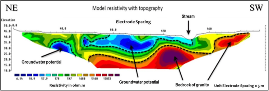
A typical resistivity cross section depicts a moderately resistive vadose zone ranging from green to orange, a less resistive saturated zone ranging blue to green, and a highly resistive confining layer ranging orange to maroon (Figure 5).

One resistivity survey line can produce a 2-D cross section (Figure 5). Multiple lines can produce a 3-D model of the site subsurface as illustrated in Figure 6. If borehole data are available, the boring logs can be overlaid on cross sections. This technique is useful for both developing a quantitative interpretation of boring log data and comparing the resistivity model to ground truth observations.

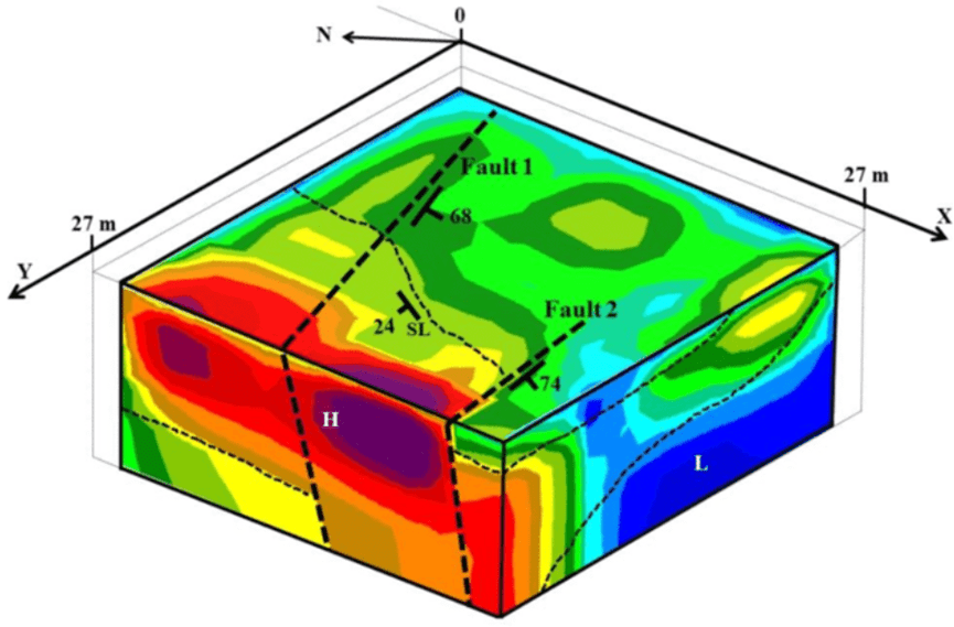
This resistivity plot locates the faults, low resistivity zone (L) indicating a water-bearing zone, and high resistivity zone (H) indicating a low permeability zone.

Like any geophysical method, resistivity benefits from knowledge of the regional and local geology for its interpretation. Depending on the goal of the survey, additional geophysical methods may be instructive as well. For instance, if the goal is to characterize contamination from buried drums, the resistivity survey could delineate the trench and plume pathways, but metal detectors or magnetometers can better locate the metal drums.

Performance Specifications

A typical line survey can interpret depths of up to 100m. Survey depth depends on the length of the survey line and the resistivity of the ground layers. Commonly used arrays (e.g., Schlumberger array and Wenner array) tend to have better vertical than horizontal resolution and are less susceptible to noise, while the dipole-dipole and pole-dipole arrays have better horizontal resolution but are more susceptible to noise. However, acquisition systems can be set up to collect hybrid arrays that improve resolution and reduce noise.

Advantages of ERT

• ERT provides broad brush, continuous, subsurface investigations across long distances (1-2 km) and covers wide areas with wide electrode spacing. It can provide short-distance, high-resolution, shallow investigation with narrow electrode spacing. There is resolution flexibility based on the setup.
• It can delineate distinct porosity and permeability zones in the subsurface to infer potential fluid pathways.
• The penetration depth is convenient for many environmental remediation applications. ERT can measure greater depths than electromagnetics, another resistivity measurement technology.
• It can be used to monitor the distribution of microbial biomass, ionic amendments, or contaminants during treatment.

Limitations of ERT

• ERT is susceptible to various sources of noise (i.e., soil and rocks, groundwater chemistry, contamination, biological activity, metallic utility lines), which can “overprint” other signals and distort the interpretation of targeted features.
• It requires sufficient space to lay a profile array while avoiding power lines, fences, buried pipe, and paved surfaces.
• It requires electrode installation.
• Tall or thick vegetation may need to be cut or disturbed to sufficiently extend the cables and set up the equipment
• People and animals must be prevented from touching the electrodes and cables during a survey to avoid electrical shocks.

Conclusion

Electrical Resistivity Tomography (ERT) is a powerful geophysical method for subsurface characterization, offering flexibility in resolution and depth penetration. While it has some limitations, its ability to provide continuous, broad-scale investigations makes it an invaluable tool in environmental and industrial applications. By understanding the theory, system components, and data interpretation techniques, users can effectively apply ERT to a wide range of subsurface challenges.

For more information on ERT and its applications, visit Geotech’s product page：

Geotech Products| Geotech Instrument Co., Ltd. (geotechcn.net)