What Is Transient Electromagnetic Method (TEM)? A Complete Technical Guide

TIPS：Transient Electromagnetic Method (TEM) maps subsurface resistivity through electromagnetic induction. This guide explains TEM physics, equipment selection, and field workflows. Geophysicists apply Transient Electromagnetic Method to groundwater, mineral, and environmental surveys. Accurate resistivity models reduce exploration risk. Subsurface resistivity data supports engineering and hydrogeological decisions.

Ⅰ. Definition and Core Principle

1. What Is TEM?

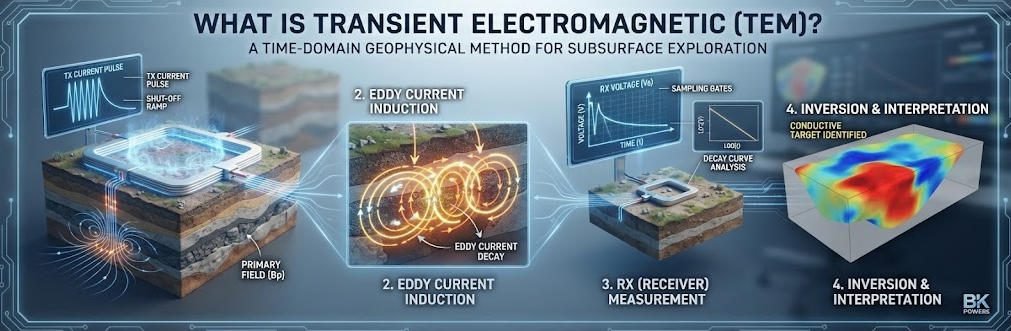
Transient Electromagnetic Method (TEM) is a time-domain geophysical technique using inductive coupling to measure subsurface electrical resistivity without ground contact. A transmitter loop emits a pulsed primary magnetic field. After current shut-off, eddy currents form in conductive ground. A receiver coil measures the decaying secondary field. This decay reveals resistivity distribution with depth.

TEM is also called Time-Domain Electromagnetics (TDEM). It requires no galvanic contact. This makes it ideal for surveys on asphalt, ice, or rock. The method excels at detecting conductive bodies in resistive host rock. It serves groundwater, mineral, and environmental exploration.

The fundamental physics follows Maxwell’s equations. Faraday’s Law governs induction. Lenz’s Law describes the opposing secondary field. Ohm’s Law relates current to conductivity. These principles combine to create the TEM response.

2. The Smoke-Ring Effect

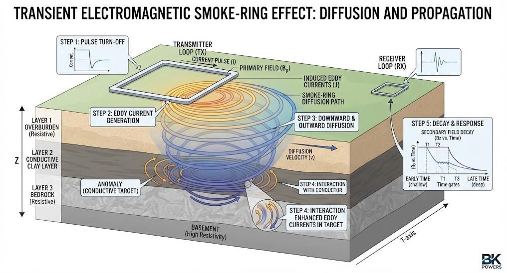
The smoke-ring concept explains TEM signal propagation. Nabighian first described this phenomenon in 1979. When transmitter current shuts off, the collapsing magnetic field induces eddy currents. These currents concentrate below the loop. They then diffuse downward and outward. The pattern resembles smoke rings rising from a cigarette.

The eddy current system expands with time. Early times correspond to shallow depths. Late times probe deeper layers. The diffusion velocity depends on ground conductivity. Conductive earth slows diffusion. Resistive earth accelerates it. This time-depth relationship enables vertical sounding.

The equivalent current filament moves downward. Its radius grows proportionally. For a homogeneous half-space, the depth of maximum current density follows the diffusion depth equation. This principle underlies all TEM interpretation.

The smoke-ring analogy is powerful. It provides an intuitive model for complex physics. Engineers use it to estimate investigation volumes. It also aids survey design. Loop size and shape influence the smoke-ring geometry.

3. Diffusion Depth and Time-Domain Behavior

TEM measures voltage decay across multiple time gates. Early gates capture nanosecond to microsecond responses. Late gates extend to milliseconds. Each gate samples a different depth interval. This temporal sampling replaces spatial arrays used in DC methods.

The diffusion depth d relates to time t and conductivity σ. It follows the approximate relation d ∝ √(t/σμ). Here μ is magnetic permeability. This square-root dependence means depth increases slowly with time. Doubling the depth requires four times the delay.

Conductive targets produce slow decay. Their secondary field persists longer. Resistive targets yield rapid decay. The signal vanishes quickly. This contrast forms the basis for anomaly detection. Interpreters analyze decay curves to identify conductive layers or bodies.

The time-domain approach offers key advantages. The primary field is absent during measurement. Only the secondary field is recorded. This eliminates primary-field noise. It allows high amplification of weak signals. The dynamic range of modern receivers exceeds 120 dB.

Ⅱ. TEM System Configurations and Equipment

1. Central-Loop Configuration

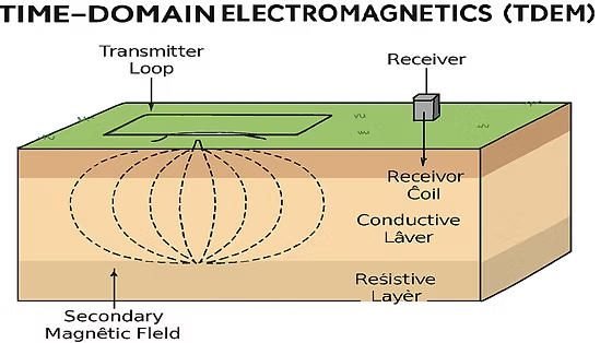
The central-loop setup places the receiver at the transmitter center. This configuration offers strong coupling. It is the most common arrangement for ground surveys. The receiver measures the vertical magnetic field component. Single-turn transmitter loops range from 20 m to 200 m per side.

Central-loop TEM provides symmetric responses. It simplifies 1D interpretation. The method works well for layered earth models. It is widely used in groundwater and mineral surveys. However, the receiver sits within the transmitter loop. This creates a shallow blind zone. Early-time data may be contaminated by turn-off transients.

The blind zone typically extends to 10–20 m depth. Fast turn-off systems reduce this zone. Some instruments achieve turn-off times below 5 microseconds. This improves shallow resolution. However, fast turn-off requires specialized transmitter electronics.

2. Fixed-Loop and Offset Configurations

Fixed-loop surveys use a large stationary transmitter. A mobile receiver moves along profiles. This setup enables rapid area coverage. The receiver can be inside or outside the loop. Offset configurations place the receiver beyond the loop edge. This avoids turn-off noise near the transmitter.

Fixed-loop methods improve lateral resolution. Multiple receiver positions sample different angles. This helps resolve dipping structures. The setup requires more complex logistics. It suits regional mapping and 3D surveys.

Offset-loop configurations reduce coupling noise. They allow earlier time measurements. This improves near-surface imaging. The trade-off is reduced signal strength. Larger transmitter currents compensate for this loss.

3. Mobile and Airborne TEM Systems

Towed TEM (tTEM) systems use continuous profiling. A transmitter and receiver array moves along the surface. This yields dense 2D coverage. Survey speeds reach several kilometers per hour. tTEM bridges the gap between discrete soundings and airborne surveys.

Airborne TEM (ATEM) mounts equipment on helicopters or fixed-wing aircraft. Large transmitter loops hang beneath the aircraft. ATEM covers vast areas rapidly. It is used for regional mineral and groundwater reconnaissance. Depth penetration is typically less than ground systems. Noise from aircraft motion and altitude limits resolution.

Waterborne TEM (wTEM) floats equipment on rivers or lakes. It maps subsurface resistivity below water bodies. USGS has deployed FloaTEM systems on multiple rivers. These map fresh-saline interfaces and aquifer geometry beneath surface water.

4. Equipment Selection Criteria

Selecting TEM equipment requires careful analysis. Target depth determines loop size and transmitter power. Shallow targets need small loops and fast turn-off. Deep targets demand large loops and high current. Geological noise and cultural interference also influence choice.

Configuration	Loop Size	Typical Depth	Best Application	Setup Time
Central-loop (portable)	20–40 m	50–200 m	Groundwater, engineering	30–60 min
Central-loop (deep)	100–200 m	200–800 m	Mineral, geothermal	1–2 hours
Fixed-loop offset	200–400 m	300–1000 m	Regional mapping	2–4 hours
Towed tTEM	10–40 m	10–150 m	Continuous profiling	Rapid
Airborne ATEM	300–500 m²	50–300 m	Regional reconnaissance	N/A

Table 1: TEM system configurations and typical performance parameters. Actual depths depend on ground resistivity and noise conditions.

Transmitter current ranges from 1 A to 50 A. Turn-off time varies from microseconds to milliseconds. Fast turn-off improves near-surface resolution. It reduces the blind zone. Receiver sensitivity and dynamic range determine signal quality. Modern systems offer 24-bit resolution and GPS synchronization.

Power supply options vary. Portable systems use rechargeable batteries. Deep systems use generators. Weight ranges from 10 kg backpack units to 100 kg+ vehicle-mounted systems. Cost scales with capability. Entry-level systems start near $20,000. Deep-penetration systems exceed $100,000.

5. TEM Historical Development

TEM methods emerged in the mid-20th century. Early systems used analog recording. The MPPO-1 appeared in 1966 for sulfide exploration. It used analog functions and proved difficult to control. North American researchers developed alternative systems. However, these struggled with late-time measurements.

Australian researchers created SIROTEM in the late 1970s. This system addressed local noise conditions. It featured larger transmitter currents and A/D converters. Other landmark systems included UTEM, Crone PEM, and Geonics EM37. These established ground TEM as a standard exploration tool.

Modern TEM instruments use digital electronics. They offer GPS synchronization and wireless communication. Real-time processing is standard. Some systems integrate with tablets or smartphones. This evolution has reduced system weight. It has also improved data quality.

6. Advanced TEM Techniques

Multi-component TEM measures multiple field components. Standard systems record the vertical component. Advanced systems add horizontal components. This improves resolution of dipping structures. It also helps distinguish geological noise from targets.

Dual-moment systems use two transmitter currents. A low moment provides early-time data. A high moment delivers late-time penetration. This combination optimizes both shallow and deep resolution. It is now standard in many commercial systems.

Borehole TEM places equipment in drill holes. This configuration investigates the volume around the hole. It detects off-hole conductors. Mining companies use this for ore body delineation. The method requires waterproof equipment. It also needs careful depth control.

Ⅲ. TEM Data Acquisition and Processing

1. Field Workflow

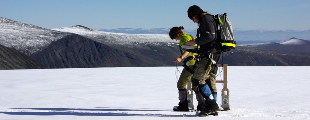
TEM field operations follow a systematic workflow. First, crews select survey stations based on target geometry. They lay out the transmitter loop on the surface. No ground penetration is needed. The receiver coil sits at the designated position. Cables connect the transmitter, receiver, and control unit.

The transmitter sends bipolar square-wave current. Typical base frequencies range from 1 Hz to 32 Hz. Lower frequencies probe deeper. Higher frequencies improve stacking efficiency. The receiver samples voltage during the off-time. Each sounding stacks hundreds to thousands of pulses. This reduces random noise.

A single sounding takes 2–10 minutes. Moving to the next station requires 5–15 minutes. Daily production reaches 15–30 soundings for ground loops. Towed systems achieve continuous profiles at walking or vehicle speed.

Survey design depends on target size and depth. Station spacing typically equals one-quarter to one-half the target depth. Lines extend beyond the target margin. This ensures adequate coverage. GPS records each station location.

2. Quality Control and Noise Management

TEM surveys face multiple noise sources. Power lines emit 50 Hz or 60 Hz interference. Radio transmitters create high-frequency noise. Moving metal objects induce spikes. Cultural features like fences and pipelines distort fields. A rule of thumb suggests keeping noise sources beyond twice the loop side length.

Quality control begins in the field. Operators monitor decay curves in real time. Noisy segments are rejected and re-measured. Stacking increases signal-to-noise ratio. Advanced systems use digital filtering and remote reference techniques. Weather conditions also matter. Lightning storms halt operations. Wind can move loops and create motion noise.

Data quality indicators include standard deviation and decay smoothness. Good data show monotonic decay. Erratic late-time points indicate noise. Experienced operators recognize these patterns. They adjust parameters to improve data quality.

3. Inversion Methods

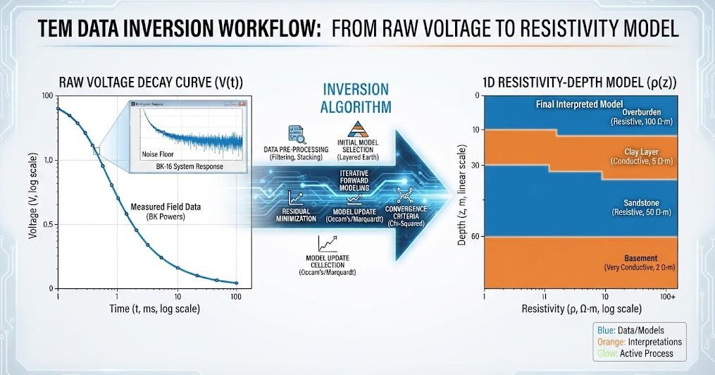
Raw TEM data are voltage-time decay curves. Inversion converts these to resistivity-depth models. One-dimensional (1D) inversion assumes horizontal layers. Each sounding yields a layered model. Multiple 1D models combine into 2D sections or 3D volumes.

Occam’s inversion minimizes model roughness. It finds the smoothest model fitting the data. This reduces non-uniqueness. Marquardt-Levenberg algorithms offer faster convergence. They work well for simple layer structures. Laterally Constrained Inversion (LCI) links adjacent soundings. It enforces geological consistency across profiles.

Two-dimensional and 3D inversion use finite-element or finite-difference methods. These handle complex geology. However, they demand significant computing power. Forward modeling validates interpretation. It simulates expected responses for proposed geological models. Comparing modeled and observed data tests hypotheses.

Processing Step	Software Approach	Output	Typical Time
Data filtering	Spike removal, stacking	Clean decay curves	Real-time
1D inversion	Occam, Marquardt	Layered resistivity model	Minutes
LCI/2D inversion	Spatial constraints	2D resistivity section	Hours
3D inversion	Finite-element mesh	3D resistivity volume	Days

Table 2: TEM data processing workflow and typical computation times.

Ⅳ. Applications by Industry

1. Groundwater and Hydrogeology

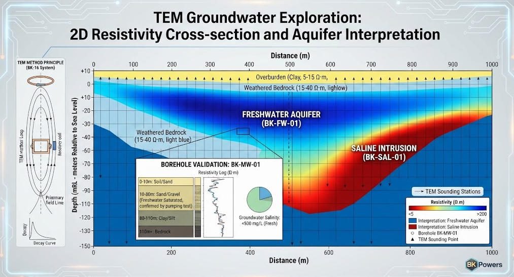
TEM is a premier tool for groundwater exploration. It maps aquifer geometry and depth. Freshwater aquifers appear resistive. Saline water or clay layers show conductive. This contrast enables aquifer delineation. TEM has mapped aquifers in volcanic islands, alluvial basins, and fractured bedrock.

Saltwater intrusion studies benefit greatly from TEM. The method maps the fresh-saline interface. This interface often lies at 10–100 m depth. TEM soundings track its lateral extent. In Oman, TDEM surveys mapped saline groundwater below 15 m across the Sea of Galilee. Resistivities below 1 Ωm indicated chloride exceeding 10,000 mg/L.

Managed Aquifer Recharge (MAR) projects use TEM for monitoring. Repeat surveys track infiltration patterns. They verify recharge facility placement. This supports climate-resilient water management. TEM also guides borehole siting in developing regions. It reduces drilling dry holes.

2. Mineral and Geothermal Exploration

TEM detects conductive sulfide mineralization. Massive sulfides yield strong responses. Disseminated ores require sensitive systems. The method penetrates conductive overburden. This is critical in regions with thick clay cover. TEM has explored for copper, gold, and base metals for decades.

Geothermal exploration uses TEM to map reservoir boundaries. Hot saline fluids within fractures create conductive anomalies. TEM identifies these zones at 300–500 m depth. When combined with AMT (Audio Magnetotelluric), the depth range extends further. The Los Humeros geothermal field employed coincident-loop TEM with 330 m loops. Soundings revealed seal-cap resistivity structure.

Deep exploration projects sometimes use grounded-wire TEM. This configuration sends current through long grounded cables. It generates different field geometries. It can achieve greater depth than loop sources. However, it requires more complex logistics.

3. Environmental and Engineering Surveys

Environmental consultants use TEM for contaminant mapping. Conductive plumes from landfills or industrial spills create detectable anomalies. TEM identifies plume extent and depth. It guides remediation drilling. This reduces investigation costs.

Engineering projects apply TEM for site characterization. It detects cavities, faults, and weak zones. Tunnel and dam projects benefit from pre-construction surveys. TEM works on paved surfaces. This avoids disruption to existing infrastructure.

Old mine workings pose safety hazards. TEM can detect water-filled voids. These appear as conductive anomalies. Mapping them prevents subsidence accidents. Rail and road projects use this capability.

Ⅴ. TEM Limitations and Method Integration

1. Physical Constraints

TEM has inherent limitations. It has a shallow blind zone. Early-time data is distorted by transmitter turn-off. This limits near-surface resolution to roughly 10–20 m. Small-loop or fast-turnoff systems reduce this zone. However, they sacrifice depth penetration.

TEM responds poorly to resistive targets in conductive hosts. A resistive ore body within conductive shale may be invisible. The method also struggles with highly conductive surface layers. Thick clay or saline soil attenuates the primary field. This reduces depth penetration.

Lateral resolution is limited. TEM soundings average over a broad area. The smoke-ring radius grows with depth. At 200 m, the effective sampling diameter may exceed 100 m. Thin vertical structures are difficult to resolve. Multi-component data and dense station spacing help. But other methods may be needed.

Topographic effects can distort data. Steep slopes alter loop geometry. This changes the primary field distribution. Corrections are possible but add complexity. Flat terrain is ideal for TEM surveys.

2. TEM and ERT Integration

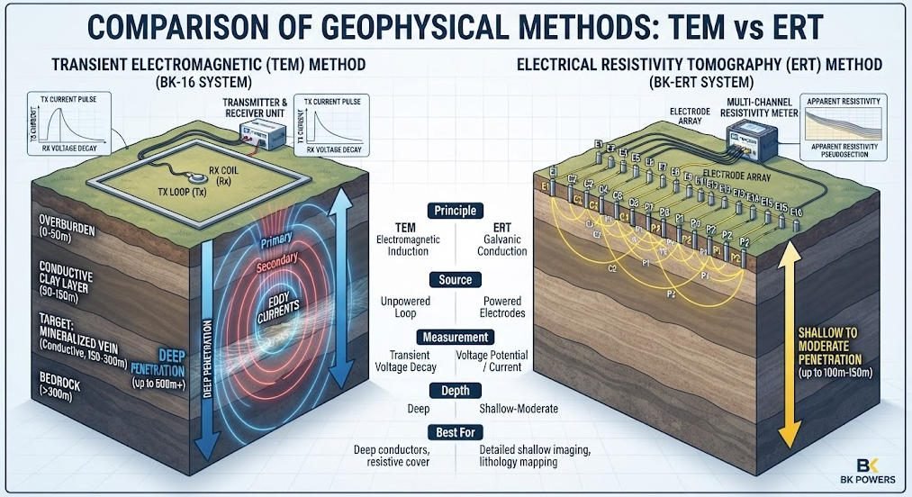
TEM and Electrical Resistivity Tomography (ERT) complement each other. ERT provides high-resolution shallow imaging. It requires galvanic contact. TEM achieves deep penetration without electrodes. The two methods overlap in the 50–150 m range. This allows cross-validation.

Integrated workflows start with TEM reconnaissance. Broad-area coverage identifies anomalies. Follow-up ERT surveys target these zones. ERT delivers detailed 2D or 3D images. This two-stage approach optimizes cost and resolution. For comprehensive site characterization, joint inversion merges both datasets.

Parameter	TEM Method	ERT Method
Principle	Electromagnetic induction	DC resistivity array
Ground contact	Not required	Required (electrodes)
Depth range	50–800+ m	10–200 m
Near-surface resolution	Poor (10–20 m blind zone)	Excellent (0.5–2 m)
Lateral resolution	Moderate	High
Setup time	30–60 min	2–4 hours
Best for	Deep conductors, regional surveys	Shallow structure, detailed imaging

Table 3: Technical comparison of TEM and ERT methods.

3. TEM and Seismic Integration

Seismic methods map structural geology. They identify faults, layers, and stratigraphy. TEM adds fluid and conductivity information. Together, they distinguish porous aquifers from tight formations. This integration is common in oil, gas, and geothermal exploration. Seismic provides the container. TEM reveals the fluid content.

Cross-hole TEM is an emerging technique. It places transmitter and receiver in boreholes. This improves resolution between holes. It is used in mining and geotechnical projects. The method requires specialized equipment. It is not yet widely available.

Ⅵ. Conclusion

Transient Electromagnetic Method remains a cornerstone of modern geophysics. Its non-invasive nature and deep penetration make it indispensable. TEM serves groundwater, mineral, environmental, and geothermal projects worldwide. Understanding its physics, limitations, and integration options ensures successful application. Geophysicists should select configurations based on target depth, geology, and project goals. When combined with ERT or seismic methods, TEM delivers robust subsurface models.

Related Articles & Resources

Title	URL
Electrical Resistivity Tomography (ERT)	https://geotechcn.net/service/what-is-electrical-resistivity-tomography-ert/
ERT vs TEM selection guide	https://geotechcn.net/service/ert-vs-tem-guide/
Cross-hole ERT and TEM integration	https://geotechcn.net/service/ert-vs-tem/
High Power IP/ERT System	https://geotechcn.net/products/electrical-instrument/high-power-ip-system/
MSATEM airborne system	https://geotechcn.net/products/em-instruments/msatem-system/
Groundwater survey techniques	https://geotechcn.net/service/how-to-conduct-a-groundwater-survey-a-technical-guide-to-accurate-results/
Electrical geophysical instruments overview	https://geotechcn.net/service/what-are-electrical-instruments/
Underground electrical exploration comparison	https://geotechcn.net/service/comparative-study-of-electrical-exploration/

Reference Sources

Title	URL
U.S. Environmental Protection Agency (EPA)	https://www.epa.gov/environmental-geophysics/time-domaintransient-electromagnetics-tdemtem
U.S. Geological Survey (USGS)	https://water.usgs.gov/ogw/bgas/methods.html
Federal Institute for Geosciences and Natural Resources (BGR)	https://www.bgr.bund.de/EN/Themen/GG_Geophysik/Bodengeophysik/Transienten_EM/tem_inhalt_en.html
ScienceDirect / Elsevier	https://www.sciencedirect.com/topics/earth-and-planetary-sciences/electromagnetic-method
Society of Exploration Geophysicists (SEG)	https://seg.org/

---

FAQ