What is ERT Testing? A Comprehensive Technical Guide

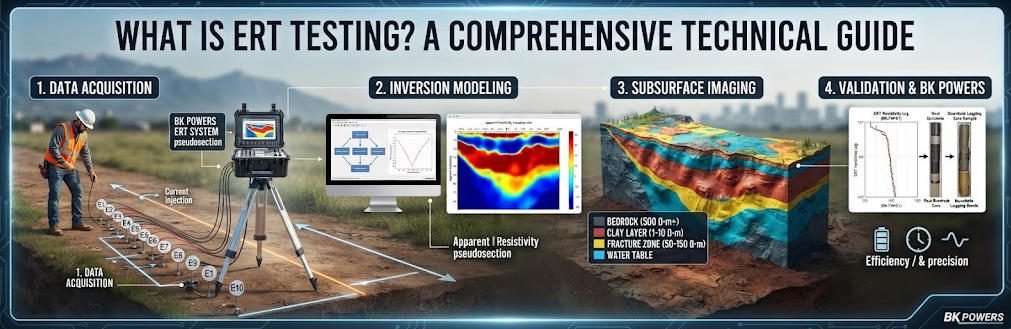
Overview：ERT testing maps subsurface resistivity using electrode arrays and direct current. This guide covers principles, array selection, and inversion workflows for ERT testing. Engineers apply electrical resistivity tomography to groundwater, mineral, and environmental surveys. Electrical resistivity tomography delivers high-resolution 2D and 3D images. Accurate data reduces drilling costs and supports geotechnical decisions.

Ⅰ. Definition and Core Principle

1. What Is ERT Testing?

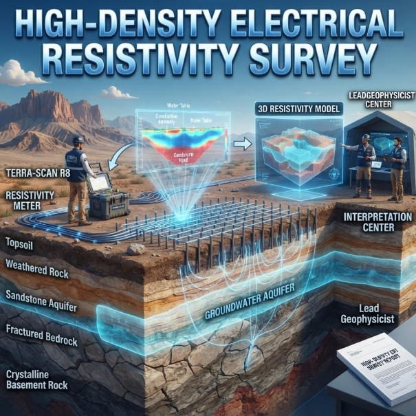
ERT testing is a geophysical method that images subsurface resistivity distribution. It uses arrays of electrodes placed along the ground surface. A resistivity meter injects direct current through two current electrodes. Two potential electrodes measure the resulting voltage difference. The instrument calculates apparent resistivity using Ohm’s Law and a geometric factor.

ERT is also called Electrical Resistivity Imaging (ERI). It combines profiling and sounding into one technique. Modern systems use 24 to 120 electrodes connected by multi-core cables. A switching unit automatically selects electrode pairs. This automation enables dense data collection without manual electrode movement.

The method requires galvanic contact. Electrodes must penetrate the ground. This limits use on paved surfaces or frozen ground. However, ERT provides exceptional spatial resolution. It resolves layers and structures as thin as 0.5 m in favorable conditions.

2. Ohm’s Law and Apparent Resistivity

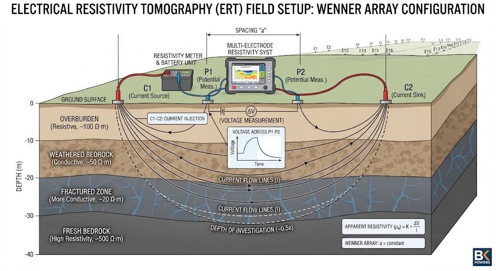
ERT testing follows Ohm’s Law. The fundamental equation is R = ΔV / I. Here R is resistance, ΔV is voltage difference, and I is current. But resistance depends on geometry. A long wire has more resistance than a short one.

Resistivity removes geometry dependence. Apparent resistivity ρa equals k × ΔV / I. The geometric factor k depends on electrode spacing and array type. For a Wenner array, k equals 2πa. Here a is the electrode spacing.

Apparent resistivity is a weighted average. It blends the resistivity of all materials between electrodes. It does not show true layer values directly. Inversion software solves this problem. It converts apparent resistivity into true resistivity models.

The relationship between current flow and electric field is governed by the continuity equation. In differential form, Ohm’s Law relates the electric field to current density and resistivity. These equations form the basis of forward modeling in ERT.

3. From DC Sounding to Tomography

Traditional DC resistivity used four electrodes per measurement. Crews moved electrodes manually. This produced 1D vertical soundings or single profiles. Data density was low. Interpretation was limited.

ERT revolutionized this approach. Multi-electrode systems collect thousands of measurements automatically. A typical 2D survey with 48 electrodes yields over 1,000 data points. The result is a continuous cross-section. This cross-section shows both lateral and vertical resistivity variations.

Three-dimensional ERT uses multiple parallel lines. Electrodes are arranged in a grid. The system collects data across all line combinations. 3D inversion produces a resistivity volume. This volume reveals complex structures like cavities, faults, and plumes.

Borehole ERT places electrodes in drill holes. This configuration investigates the volume between holes. It achieves higher resolution at depth. Cross-hole ERT is used in mining and geotechnical projects. It requires waterproof electrode strings.

Ⅱ. Electrode Arrays and Survey Design

1. Wenner Array

The Wenner array uses equal spacing between all four electrodes. Current electrodes sit at the ends. Potential electrodes sit in the middle. All four electrodes move together. The spacing a increases for deeper measurements.

Wenner arrays provide strong signals. They work well in noisy environments. The horizontal resolution is good for layered earth. However, the array requires more field labor. Each depth level needs physical electrode movement.

The geometric factor is simple. k = 2πa. This simplicity aids quality control. Signal strength is high because potential electrodes are close to current electrodes. The array is less sensitive to lateral variations. It is best for 1D sounding and layered structures.

2. Schlumberger Array

The Schlumberger array keeps potential electrodes fixed. Only current electrodes move outward. The potential spacing MN is small compared to current spacing AB. This reduces field labor. It also improves vertical resolution.

The geometric factor is more complex. It depends on both AB and MN spacing. The array provides good depth penetration. It is widely used for vertical electrical sounding (VES). Many hydrogeological surveys use Schlumberger configurations.

Wenner-Schlumberger hybrid arrays combine both approaches. These are common in modern ERT systems. They balance signal strength and data density. The hybrid array is the default choice for many commercial instruments.

3. Dipole-Dipole Array

The dipole-dipole array separates current and potential pairs. Each pair has a fixed spacing a. The separation between pairs is n times a. The factor n increases for deeper measurements.

This array offers excellent lateral resolution. It detects steeply dipping structures and faults. It is ideal for complex geology. However, signal strength decreases rapidly with n. Noise becomes a problem at large separations.

The array is less sensitive to horizontal layers. It may miss subtle vertical contacts. Many surveys combine dipole-dipole with Wenner data. This combination improves overall resolution.

4. Array Selection Criteria

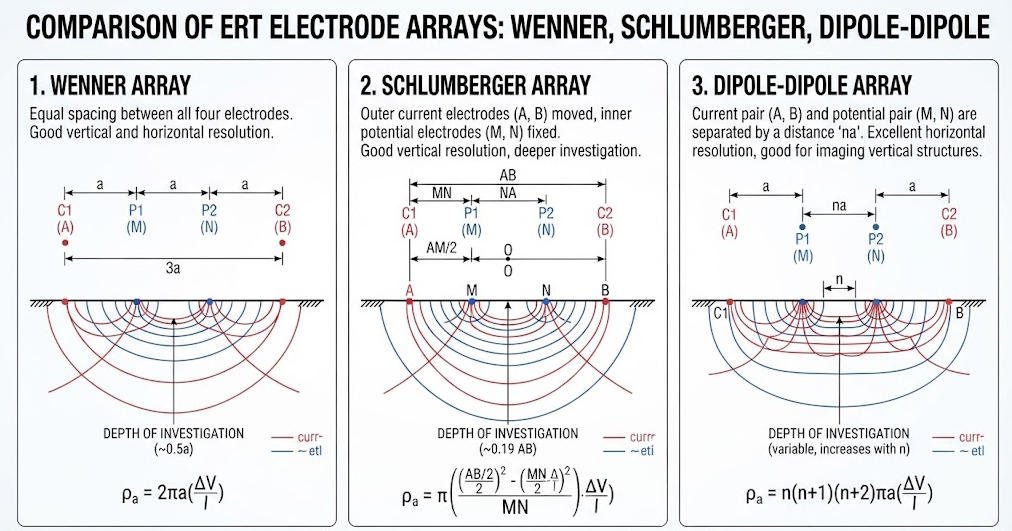
Selecting the right array requires careful analysis. Target geometry, depth, and noise conditions all matter. The table below summarizes key differences.

Array Type	Signal Strength	Vertical Resolution	Lateral Resolution	Best Application
Wenner	High	Good	Moderate	Layered geology, 1D sounding
Schlumberger	High	Very good	Moderate	Deep VES, hydrogeology
Dipole-Dipole	Low to moderate	Moderate	Excellent	Faults, cavities, steep structures
Wenner-Schlumberger	High	Good	Good	General 2D/3D ERT surveys

Table 1: Comparison of common ERT electrode arrays. Signal strength and resolution vary with geological conditions and instrument capability.

Survey design also depends on target depth. A rule of thumb states that profile length should be three to five times the target depth. Electrode spacing determines near-surface resolution. Closer spacing improves detail but reduces depth penetration.

For groundwater exploration, 5 m electrode spacing is common. This achieves approximately 40 m depth with Wenner-Schlumberger arrays. For engineering surveys, 1 to 2 m spacing resolves shallow structures. For deep mineral exploration, 10 to 20 m spacing extends penetration.

5. Resistivity Ranges for Common Geological Materials

Interpretation requires knowledge of typical resistivity values. Igneous and metamorphic rocks generally range from 1,000 to 10,000 Ωm. Sedimentary rocks show intermediate values from 10 to 1,000 Ωm. Unconsolidated sediments typically range from 10 to 100 Ωm. Clay and saline water fall below 10 Ωm. These ranges guide initial interpretation. Local conditions may shift values significantly.

Water content strongly affects resistivity. Saturated sand shows lower resistivity than dry sand. Temperature also matters. Warm groundwater is more conductive than cold water. Mineralization increases conductivity. High chloride content reduces resistivity dramatically.

6. Equipment Selection

ERT instruments vary in capability. Entry-level systems use 24 electrodes. Research-grade systems deploy 120 or more. Channel count determines measurement speed. Multi-channel systems collect data faster than single-channel units.

Power output affects depth penetration. Standard systems use 200 to 400 V. High-power systems reach 1,000 V or more. These penetrate deeper but require safety precautions. Current output ranges from tens of milliamps to several amps.

Portability is another factor. Backpack systems suit remote areas. Vehicle-mounted systems handle large surveys. Wireless systems reduce cable clutter. They improve efficiency in difficult terrain.

Ⅲ. Data Acquisition and Processing

1. Field Workflow

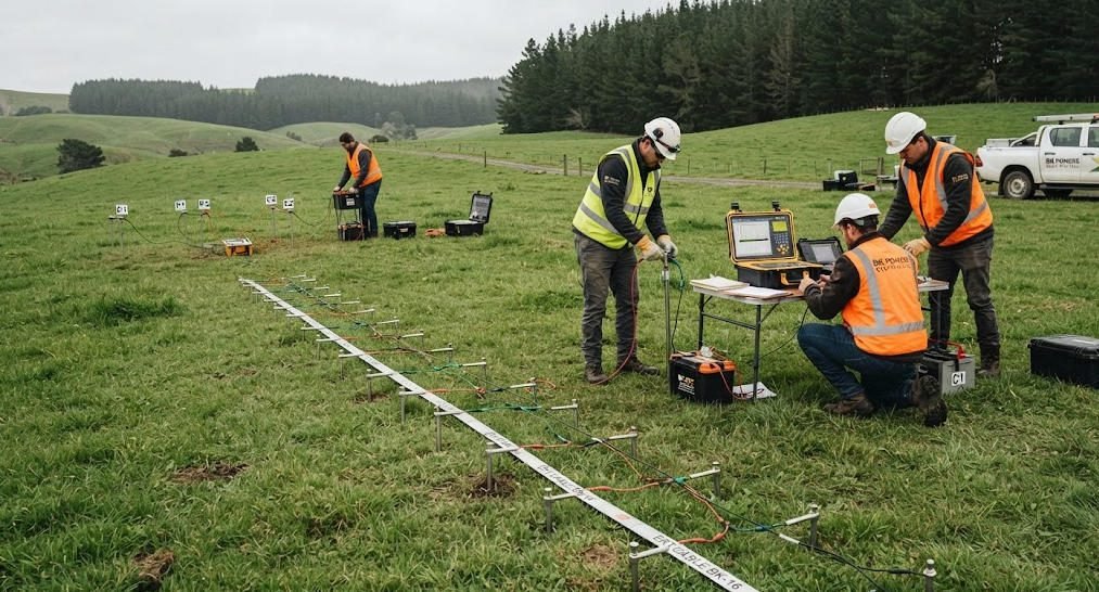
ERT field operations follow a systematic procedure. First, crews lay out the electrode line. They use a tape measure for accurate spacing. Electrodes are driven 10 to 20 cm into the ground. This ensures good galvanic contact.

Next, cables connect electrodes to the switching unit. The resistivity meter sends current and records voltage. Modern systems automate this process. They cycle through hundreds of electrode combinations. A complete dataset takes 15 minutes to 2 hours.

Topography matters. Sloping terrain distorts current flow. Most inversion software includes topographic correction. GPS or total station data provides elevation profiles. Correcting for topography improves model accuracy.

Weather conditions affect data quality. Rain reduces contact resistance. It can also create near-surface conductive layers. Dry conditions increase contact resistance. Crews may need to water electrodes.

2. Quality Control

Data quality depends on electrode contact. Dry or rocky soil increases contact resistance. Crews may add salt water or bentonite mud around electrodes. This improves conductivity. Regular contact resistance checks are essential.

Noise sources include power lines, fences, and pipelines. A rule of thumb suggests keeping the survey line away from these features. The distance should exceed the maximum electrode spacing. Metal objects near the line cause data distortion.

Stacking reduces random noise. Each measurement repeats several times. The instrument averages the results. Stacking factors of 2 to 8 are common. Higher stacking improves quality but increases survey time.

Data filtering removes bad points. Erratic readings often indicate poor contact or nearby metal. Inversion software flags outliers. Experienced operators review these flags. They decide whether to delete or keep questionable data.

3. Inversion Methods

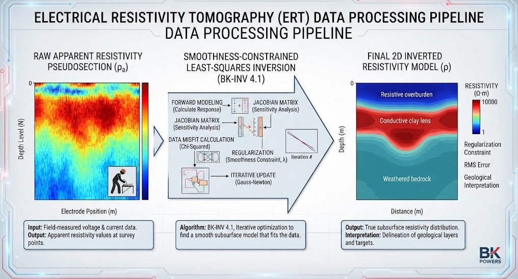
Raw ERT data are apparent resistivity values. Inversion converts these to true resistivity models. The process is mathematically non-unique. Multiple models can fit the same data. Regularization stabilizes the solution.

Smoothness-constrained least-squares inversion is the standard approach. It minimizes model roughness while fitting data. The result is a geologically realistic image. L2-norm regularization produces smooth transitions. L1-norm sharpens boundaries.

Occam’s inversion finds the simplest model that fits data. It avoids over-interpretation. Gauss-Newton methods offer faster convergence. They work well for large datasets. Advanced software uses finite-element or finite-difference forward modeling.

The pseudosection is an intermediate product. It plots apparent resistivity against electrode position and spacing. Pseudosections provide a first look at data quality. They reveal obvious anomalies and noise patterns. However, they are not true depth sections. Inversion is required for accurate interpretation.

Processing Step	Method	Output	Typical Duration
Data filtering	Outlier removal, stacking	Clean apparent resistivity dataset	Real-time to 1 hour
Pseudosection	Apparent resistivity plotting	Preliminary quality assessment	Minutes
2D inversion	Smoothness-constrained least-squares	2D resistivity cross-section	5–30 minutes
3D inversion	Finite-element or finite-difference	3D resistivity volume	1–8 hours
Time-lapse inversion	Difference inversion	Change detection images	Hours to days

Table 2: ERT data processing workflow and typical computation times. Duration depends on data volume and computer hardware.

Ⅳ. Applications by Industry

1. Groundwater and Hydrogeology

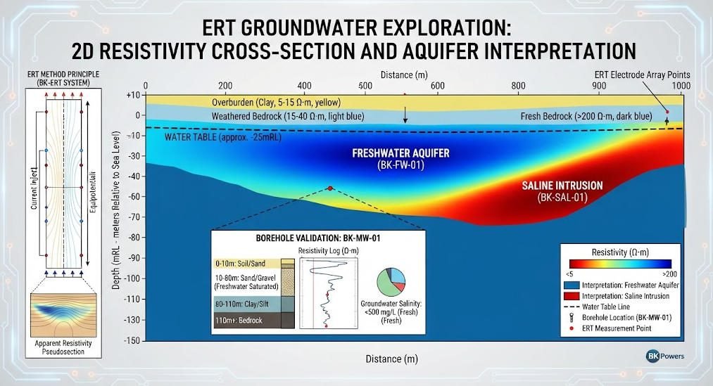
ERT is a premier tool for groundwater exploration. Freshwater aquifers show resistive signatures. Clay layers and saline water appear conductive. This contrast enables aquifer mapping. ERT delineates aquifer geometry and depth.

Saltwater intrusion studies use ERT extensively. The fresh-saline interface creates a sharp resistivity contrast. ERT tracks this interface over time. Repeat surveys monitor intrusion progression. This supports coastal water management.

In fractured rock terrains, ERT identifies water-bearing zones. However, interpretation is challenging. Fractured sandstone and clay-rich rocks can show similar resistivity. Borehole validation is essential. Depending on geological conditions, ERT alone may not distinguish these lithologies.

Time-lapse ERT monitors infiltration and recharge. Repeat surveys at the same location track resistivity changes. Wetting fronts appear as conductive anomalies moving downward. This supports managed aquifer recharge design.

2. Mineral and Mining Exploration

ERT detects sulfide mineralization. Massive sulfides are highly conductive. They create strong low-resistivity anomalies. Disseminated ores are harder to resolve. They may require combined ERT and IP surveys.

Mine void detection is another key application. Abandoned workings fill with water or air. Water-filled voids appear conductive. Air-filled voids appear resistive. ERT maps these hazards before construction or mining operations.

Tailings dam monitoring uses time-lapse ERT. Repeat surveys track moisture changes. They detect seepage paths and potential failures. This supports mine safety and environmental compliance.

3. Environmental and Engineering Surveys

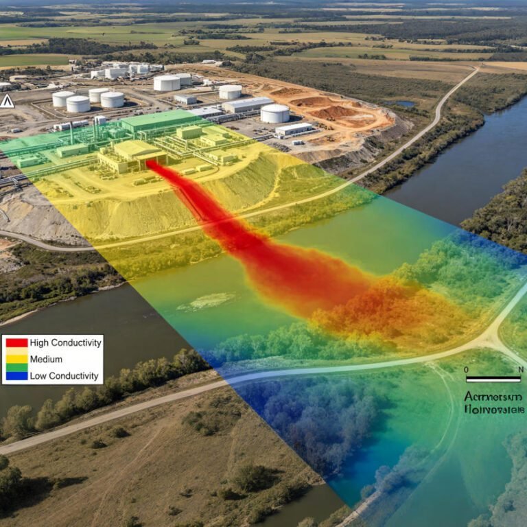
Environmental consultants use ERT for contaminant mapping. Conductive plumes from landfills or spills create detectable anomalies. ERT identifies plume extent and depth. It guides remediation drilling. This reduces investigation costs.

Karst terrain investigations benefit from ERT. Cavities and sinkholes show resistive signatures. ERT profiles across suspected zones reveal subsurface voids. Engineers use this data to assess foundation stability.

Road and dam projects apply ERT for site characterization. It detects weak zones, faults, and saturated layers. Pre-construction surveys prevent costly surprises. ERT works well in conjunction with seismic methods.

Landslide studies use ERT to map the slip surface. Saturated zones at the base of slopes appear conductive. ERT identifies these weak layers. This supports slope stability assessment and mitigation design.

Ⅴ. Method Integration and Limitations

1. ERT and VES Integration

ERT and Vertical Electrical Sounding (VES) complement each other. VES provides 1D depth information at single points. It uses Schlumberger or Wenner arrays. VES is faster and cheaper for reconnaissance.

ERT provides 2D or 3D spatial coverage. It resolves lateral variations. Integrated workflows start with VES reconnaissance. VES soundings identify key depths and resistivity ranges. Follow-up ERT surveys target anomalous zones.

In the Enugu metropolis of Nigeria, researchers combined VES and 2D ERT for groundwater exploration. VES used Schlumberger arrays. ERT used Wenner configurations. The combination improved aquifer delineation. Water table depth was determined at 18 m. Maximum drill depth reached 100 m.

Parameter	ERT Method	VES Method
Dimensionality	2D or 3D	1D
Spatial coverage	Continuous profile	Single point
Electrodes	24–120+	4
Setup time	1–3 hours	30–60 minutes
Best for	Lateral variation mapping	Depth reconnaissance

Table 3: Technical comparison of ERT and VES methods.

2. ERT and IP Integration

Induced Polarization (IP) measures chargeability. It detects the temporary storage of electrical energy in rocks. IP is highly sensitive to sulfide minerals and clay content. ERT measures resistivity. Together, they provide complementary information.

IP and ERT use the same electrode arrays. Specialized resistivity meters collect both datasets simultaneously. Chargeability data enhances mineral exploration. It identifies disseminated sulfides that resistivity alone may miss.

In Canada, researchers integrated ERT and IP to map Pb-Zn-Ag sulfide deposits. ERT revealed resistivity ranges of 700–2,000 Ωm. IP showed chargeability values of 3.5 mV/V. The combined approach successfully delineated ore boundaries at 80–150 m depth. Borehole logs validated the results.

3. Physical Constraints

ERT has inherent limitations. It requires galvanic contact. Dry sand, asphalt, and frozen ground block current injection. Alternative methods like GPR or TEM may be needed in these conditions.

Depth penetration is limited. Resolution decreases exponentially with depth. Highly resistive materials attenuate current. This reduces signal quality. Depending on geological conditions, maximum practical depth ranges from 50 m to 200 m for most surface arrays.

Lateral resolution depends on electrode spacing. Small features between electrodes may be missed. The method averages resistivity over the measurement volume. Thin vertical structures are difficult to resolve.

Topographic effects distort data. Steep slopes alter current flow patterns. Software corrections help but add uncertainty. Flat terrain is ideal for ERT surveys.

Electrical noise from power lines and metal structures degrades data. Surveys near urban infrastructure require careful planning. Nighttime measurements sometimes reduce power line interference.

Ⅵ. Conclusion

ERT testing remains a cornerstone of near-surface geophysics. Its ability to image subsurface resistivity in 2D and 3D makes it indispensable. The method serves groundwater, mineral, environmental, and engineering projects worldwide.

Successful ERT surveys depend on proper array selection and survey design. Understanding the target geometry and geological context ensures meaningful results. Integration with VES, IP, or seismic methods reduces interpretation ambiguity.

Geophysicists should follow established standards such as ASTM D6431 for field procedures. Quality control during acquisition and careful inversion produce reliable models. When applied correctly, ERT testing delivers robust subsurface characterization that supports drilling decisions and engineering design.

Related Articles

Title	Core Content	URL
What is Electrical Resistivity Tomography (ERT)?	Comprehensive ERT fundamentals, Ohm’s Law, and 3D imaging principles	https://geotechcn.net/service/what-is-electrical-resistivity-tomography-ert/
What is Vertical Electrical Sounding (VES)?	VES principles, Schlumberger arrays, and depth sounding methodology	https://geotechcn.net/service/what-is-vertical-electrical-sounding-ves/
ERT vs TEM Guide	Technical comparison of ERT and transient electromagnetic methods for deep exploration	https://geotechcn.net/service/ert-vs-tem-guide/
Wenner Array Guide	Wenner array configuration, geometric factor, and high-density resistivity imaging	https://geotechcn.net/service/ert-wenner-array/
Groundwater Survey Technical Guide	Step-by-step methodology for conducting hydrogeophysical surveys with ERT	https://geotechcn.net/service/how-to-conduct-a-groundwater-survey-a-technical-guide-to-accurate-results/
Electrical Geophysical Instruments Overview	Classification and selection of DC resistivity, IP, and ERT instruments	https://geotechcn.net/service/what-are-electrical-instruments/
Comparative Study of Electrical Exploration	Integrated comparison of ERT, VES, IP, and electromagnetic methods	https://geotechcn.net/service/comparative-study-of-electrical-exploration/
High Power IP System	Deep induced polarization and resistivity measurement system specifications	https://geotechcn.net/products/electrical-instrument/high-power-ip-system/

Reference Sources

Title	Core Content	URL
USGS — Principles of Surface Geophysical Techniques: DC Resistivity	Federal guidance on DC resistivity fundamentals, electrode configurations, and fracture detection applications	https://water.usgs.gov/ogw/bgas/surface/
US EPA — Electrical Resistivity	Environmental applications of electrical resistivity methods for groundwater, contamination, and site characterization	https://www.epa.gov/environmental-geophysics/electrical-resistivity
ASTM D6431-25 — Standard Guide for Using the Direct Current Resistivity Method	International standard for DC resistivity field procedures, equipment, and interpretation in geophysical site investigation	https://www.astm.org/d6431-25.html
DOE — Imaging Goes Underground at the Hanford Site	DOE case study on time-lapse ERT monitoring for polyphosphate remediation using PNNL E4D software	https://www.energy.gov/em/articles/imaging-goes-underground-hanford-site
FRTR — Electrical Resistance Tomography for Soil	Federal remediation technology review of ERT applications at DOE and DOD sites including LLNL and Savannah River	https://frtr.gov/costperformance/monitoring/

---

FAQ