Welcome to Geotech!
-1.png)

What is EM Resistivity: Principles, 2D/3D Imaging Methods
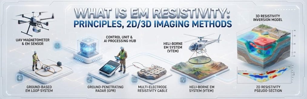
Overview:This guide explores electrical resistivity tomography fundamentals for near-surface geophysical investigation. It details electrical resistivity tomography workflows, evaluates 2D/3D resistivity imaging performance, and compares 2D/3D resistivity imaging tradeoffs across mining, geotechnical and infrastructure engineering scenarios.
Ⅰ. Definition and Core Principles
1. Core Definition
Electrical resistivity methods are non-invasive geophysical techniques that map subsurface resistivity distribution via controlled current injection and surface voltage measurement. They detect contrasts in electrical properties between different subsurface materials and formations. The technology supports 1D depth profiling, 2D cross-sectional imaging and full 3D volumetric modeling.
2. Physical Measurement Principle
The measurement follows Ohm’s Law: V = I × R, where V is measured potential difference and I is injected current. A standard four-electrode configuration uses two outer current electrodes and two inner potential electrodes. This arrangement eliminates contact resistance errors from the measurement chain. Apparent resistivity is calculated as ρₐ = K × (V/I), where K is a geometric factor determined by electrode spacing.
Apparent resistivity represents a weighted average of all materials within the current flow volume. It differs from true formation resistivity because the subsurface is never perfectly homogeneous. Inversion processing converts apparent resistivity values into accurate subsurface resistivity distributions. Advanced inversion algorithms produce geologically realistic models for engineering interpretation.
3. Core Method Taxonomy
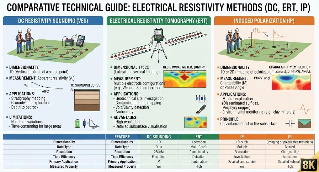
Three primary resistivity-based methods serve different survey objectives and depth ranges. Each delivers distinct dimensionality, resolution and depth capability.
| Method | Measurement Dimensionality | Core Mechanism | Primary Application |
|---|---|---|---|
| Electrical Resistivity Tomography (ERT) | 2D / 3D | Dense multi-electrode switching | High-resolution near-surface imaging |
| DC Resistivity Sounding (VES) | 1D | Expanding electrode spacing | Deep vertical stratigraphic profiling |
| Induced Polarization (IP) | 2D / 3D | Transient voltage decay | Mineral and contaminant characterization |
ERT provides the highest spatial resolution for detailed near-surface imaging. DC sounding delivers the greatest depth penetration for vertical stratigraphic information. Induced polarization adds electrochemical data for mineral identification and contaminant characterization.
Ⅱ. 2D vs 3D Resistivity Imaging
1. 2D Electrical Resistivity Tomography
2D ERT deploys electrodes along a single linear survey line. It produces cross-sectional resistivity slices perpendicular to the ground surface. The method assumes approximate lateral homogeneity perpendicular to the survey line. This simplifies acquisition and reduces both field time and processing cost.
2D surveys deliver cost-effective linear profiling for corridor-style projects. They work well for elongated targets such as faults, dikes and utility corridors. Common applications include railway foundation assessment, fault zone mapping and pipeline alignment surveys. The primary limitation is poor performance with complex 3D structures like karst caves or irregular ore bodies.
2. 3D Electrical Resistivity Tomography
3D ERT uses grid, cross-line or rectangular electrode layouts to acquire volumetric data. It produces true 3D resistivity distributions that accurately represent complex subsurface geometries. Pseudo-3D configurations use parallel 2D lines with interpolation for cost-effective volumetric approximation. True 3D grid arrays deliver the highest spatial accuracy but require significantly more electrodes.
3D imaging enables precise spatial modeling of complex targets like goaf zones, karst conduits and irregular ore bodies. It eliminates interpretation ambiguity associated with off-line structures. The main challenges include higher equipment cost, longer acquisition time and greater computational demands. Advanced algorithms like finite element modeling and Occam inversion are required for large 3D datasets.
3. Comparative Performance Matrix
The following matrix compares key performance parameters across 2D, pseudo-3D and true 3D configurations. This reference supports method selection based on project objectives and budget constraints.
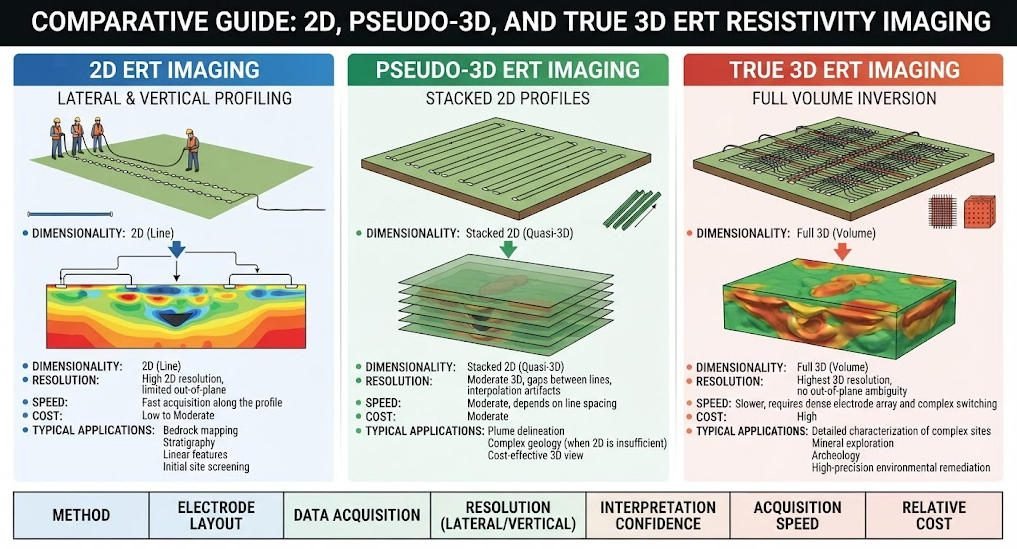
| Parameter | 2D ERT | Pseudo-3D ERT | True 3D ERT |
|---|---|---|---|
| Electrode Layout | Single linear line | Parallel 2D lines | Rectangular grid array |
| Spatial Dimensionality | 2D cross-section | Quasi-3D volume | Full 3D volume |
| Lateral Resolution | 0.5–3 m along line | 1–5 m in-line, 5–10 m cross-line | 0.5–3 m isotropic |
| Relative Acquisition Speed | High | Medium | Low |
| Processing Complexity | Low | Medium | High |
| Relative Survey Cost | Low | Medium | High |
| Best For | Linear corridors, faults | Regional volumetric screening | Complex 3D targets, detailed modeling |
Ⅲ. Forward Modeling and Inversion Algorithms
1. Forward Modeling Approaches
Forward modeling calculates theoretical surface response for a given subsurface resistivity model. It is a core component of the inversion process. Two primary approaches are used in engineering practice.
Finite Element Method (FEM) delivers high accuracy for complex terrains and irregular topography. It handles variable surface elevation and complex subsurface geometries effectively. The main drawback is high computational cost, especially for large 3D models.
Analytical solutions provide exact results for simple layered earth models. They are computationally efficient and serve as educational tools and initial test cases. Their application is limited to horizontally layered media with no lateral variation.
2. Inversion Algorithm Classification
Inversion converts measured apparent resistivity data into true subsurface resistivity distributions. It solves an ill-posed problem with multiple mathematically valid solutions. Regularization techniques add constraints to produce geologically reasonable results.
Regularized inversion using L1 and L2 norms represents the standard engineering approach. L2 norm regularization imposes smoothness constraints, producing continuous resistivity models. It is numerically stable and widely adopted for routine survey interpretation. L1 norm regularization favors sparse solutions with sharper boundaries between units. It better resolves sharp electrical contrasts like fault zones and cavity boundaries.
Occam inversion constructs the simplest possible model that fits the data within error tolerance. It follows the principle of minimum structure, producing smooth models with minimal complexity. This approach is widely valued for its robustness and reliability in exploration applications.
3. Regularization and Stability
Regularization balances data fit and model plausibility in underdetermined inverse problems. The regularization factor λ controls the relative weight of data misfit and model constraint. Proper selection of λ is critical for producing accurate, geologically realistic results.
Adaptive regularization methods adjust λ through the inversion process. Ratio methods and step-decay methods prevent early convergence to singular solutions. This improves inversion stability and reduces dependence on initial model selection.
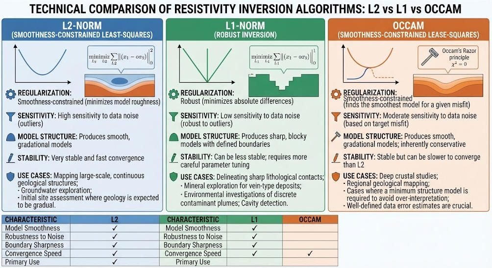
| Approach | Core Principle | Resolution Characteristic | Primary Use Case |
|---|---|---|---|
| L2 Norm Regularization | Smoothness constraint | Gradual boundaries, blurred contacts | General engineering surveys |
| L1 Norm Regularization | Sparsity constraint | Sharp boundaries, block-like features | Faults, cavities, discrete targets |
| Occam Inversion | Minimum structure principle | Smooth, conservative models | Regional exploration, reconnaissance |
Ⅳ. Field Applications and Engineering Case Studies
1. Mining and Goaf Detection
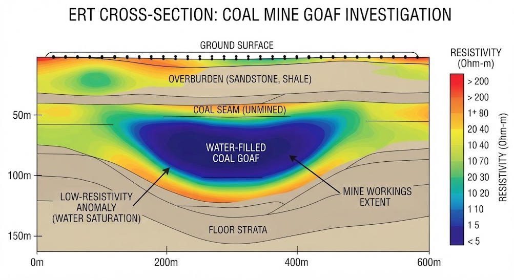
Resistivity imaging reliably detects water-filled goaf zones in coal mining areas. Water-filled voids produce distinct low-resistivity anomalies against higher-resistivity bedrock. Pseudo-3D survey designs provide cost-effective volumetric coverage of mining concessions.
In Hubei coal fields, WGMD-9 systems deployed Wenner array configurations for goaf detection. Pseudo-3D inversion successfully mapped boundaries of water-filled abandoned workings. Low-resistivity anomalies correlated well with known mine workings confirmed by subsequent drilling. This approach supports safe mine planning and subsidence hazard assessment.
2. Karst and Geotechnical Engineering
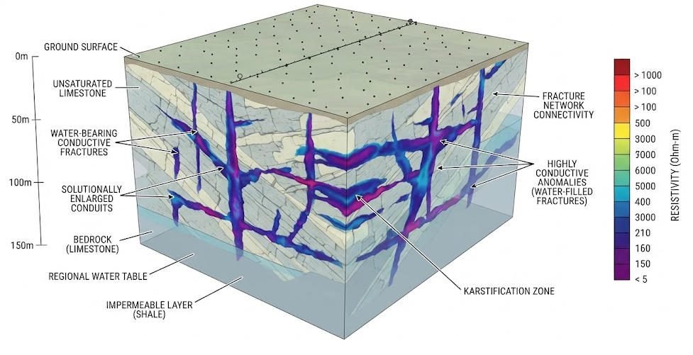
ERT is a standard tool for karst characterization in limestone and carbonate terrains. It detects water-filled fissures, dissolution conduits and bedrock integrity variations. High resistivity values indicate intact bedrock, while low resistivity marks water-bearing fracture zones.
In Guangdong limestone areas, ERT surveys delineated dissolution fissure networks for foundation design. Results guided pile foundation design and ground improvement programs. The method identified both major conduits and diffuse fracture zones affecting construction stability. This reduces foundation risk and optimizes ground treatment costs.
3. Utility and Infrastructure Mapping
Resistivity methods detect both metallic and non-metallic underground utilities. Non-metallic pipes like PVC present particular challenges for many geophysical methods. Dipole-dipole array configurations enhance sensitivity to small, discrete subsurface features.
Proper array selection significantly improves detection rates for non-conductive utilities. Dipole-dipole arrays produce better lateral resolution of small diameter targets. Survey design must account for target depth, size and expected resistivity contrast. This ensures reliable detection for utility locating and pre-construction clearance surveys.
Ⅴ. Performance, Advantages and Limitations
1. Effective Depth and Resolution
Effective investigation depth depends on electrode array spread, transmitter power and ground resistivity. Standard ERT systems typically achieve 5 to 300 meters of effective depth. Depth equals approximately one-fifth to one-third of total electrode array spread. Spatial resolution decreases exponentially with increasing depth across all configurations.
Lateral resolution depends on electrode spacing and array type. Standard surveys achieve 0.5 to 3 meters resolution at shallow to intermediate depths. Deeper targets produce proportionally lower resolution images. Resolution also varies with target contrast and geological complexity.
2. Key Advantages
Electrical resistivity methods are non-destructive and require only minimal ground disturbance. This makes them suitable for sensitive sites like archaeological locations and protected ecosystems. They provide continuous subsurface profiles between widely spaced boreholes.
Multi-parameter fusion with induced polarization adds mineralogical and electrochemical information. This combined approach improves detection of clay zones, contaminant plumes and sulfide mineralization. It reduces interpretation ambiguity compared to single-parameter resistivity surveys.
3. Limitations and Mitigation
Standard ERT has effective depth limitations typically below 200 meters for most engineering configurations. Current decay with depth reduces signal strength at greater depths. High-power systems can extend depth in resistive formations.
Topographic effects on steep slopes can produce data artifacts. Topographic correction algorithms compensate for elevation variations along survey lines. Rugged terrain surveys require careful survey design and data processing adjustments.
Cultural noise from power lines, pipelines and infrastructure can degrade data quality. Filtering techniques, electrode layout optimization and repeat measurements mitigate noise effects. Urban surveys typically use Wenner arrays for higher signal-to-noise ratio.
Related Articles
| Title | Core Content | URL |
|---|---|---|
| What is Electrical Resistivity Tomography (ERT)? | ERT principles, electrode acquisition, 2D/3D resistivity modeling | https://geotechcn.net/service/what-is-electrical-resistivity-tomography/ |
| Electrical Resistivity Tomography: A Complete Technical Guide | ERT fundamentals, electrode configurations, inversion and applications | https://geotechcn.net/service/electrical-resistivity-tomography-a-complete-technical-guide/ |
| Resistivity Surveying Techniques | High-density resistivity, DC sounding, 2D/3D ERI and method comparison | https://geotechcn.net/service/resistivity-surveying-techniques/ |
| What Is an ERT Instrument? | ERT instruments, high-density resistivity, DC sounding and acquisition systems | https://geotechcn.net/service/ert-instruments/ |
| What is Induced Polarization (IP) Method? | IP physical principles, chargeability, applications and resistivity-IP comparison | https://geotechcn.net/service/what-is-induced-polarization-ip-method/ |
| What is a Multi-Electrode System? | Multi-electrode acquisition, 2D/3D imaging and high-density electrical methods | https://geotechcn.net/service/what-is-a-multi-electrode-system-exploring-2d-3d-resistivity-imaging-applications/ |
| 2D vs 3D Electrical Resistivity Imaging | Differences between linear 2D imaging and volumetric 3D imaging | https://geotechcn.net/service/2d-vs-3d-electrical-resistivity-imaging-methods/ |
| What is ERT Equipment? | ERT system architecture, acquisition, processing and equipment concepts | https://geotechcn.net/service/what-is-ert-equipment/ |
Reference Sources
| Title | Core Content | URL |
|---|---|---|
| ASTM D6431-25 — Standard Guide for Using the Direct Current Resistivity Method for Geophysical Site Investigation | DC resistivity principles, equipment, electrode arrays, apparent resistivity, ERT/ERI inversion, 2D/3D interpretation and safety | http://store.astm.org/d6431-25.html |
| US EPA — Electrical Resistivity | Four-electrode measurement, apparent resistivity, geometric factor, electrode arrays and depth of investigation | http://www.epa.gov/environmental-geophysics/electrical-resistivity |
| US EPA — Electrical Methods | Distinguishes galvanic electrical methods from inductive electromagnetic methods and explains subsurface electrical properties | http://www.epa.gov/environmental-geophysics/electrical-methods |
| USGS — Electrical Imaging for Hydrogeology | Electrical imaging theory, hydrogeological applications, field practice, inversion and QA/QC | http://www.usgs.gov/publications/electrical-imaging-hydrogeology |
| US EPA — Inversion | Forward and inverse problems, non-uniqueness, instability, noise and geophysical model estimation | http://www.epa.gov/environmental-geophysics/inversion |
FAQ
Q1: What is electrical resistivity tomography (ERT)?
ERT is a non-invasive geophysical technique that maps subsurface resistivity using electrode arrays and controlled current injection. It measures voltage response and uses inversion algorithms to produce 2D or 3D resistivity models. Four-electrode configurations eliminate contact resistance errors. It is widely used for geotechnical site characterization, karst detection and mining goaf mapping.
Q2: What is the difference between 2D and 3D ERT?
2D ERT produces cross-sectional slices along single survey lines, while 3D ERT generates volumetric resistivity models. 2D assumes lateral homogeneity and costs less; 3D uses grid arrays for isotropic resolution but requires more electrodes and computing. Pseudo-3D offers a middle ground with parallel lines. 2D suits linear corridors; 3D is preferred for complex targets like karst caves.
Q3: What inversion algorithms are used for resistivity data?
Standard approaches include L2 norm, L1 norm and Occam inversion with different regularization characteristics. L2 produces smooth models, L1 favors sharp boundaries, and Occam generates minimum-structure solutions. Regularization balances data fit and model plausibility for the ill-posed inverse problem. L2 is standard for general engineering; L1 improves fault and cavity detection.
Q4: How deep can electrical resistivity surveys effectively detect?
Standard ERT achieves 5–300 meters effective depth depending on array spread and transmitter power. Depth equals roughly one-fifth to one-third of total electrode array spread. Current decay with depth limits maximum penetration. High-power systems extend depth in resistive formations. Standard engineering surveys target the upper 100 meters.
Q5: What are the main advantages of ERT over other methods?
ERT provides continuous subsurface imaging with minimal ground disturbance and works well in clay soils where GPR fails. It delivers good resolution at intermediate depths and supports multi-parameter fusion with induced polarization. The non-destructive nature suits sensitive archaeological and environmental sites. It is ideal for karst hazard assessment and dam seepage monitoring.